Multivariate analyses
Last compiled on oktober, 2024
Getting started
To copy the code, click the button in the upper right corner of the code-chunks.
clean up
rm(list = ls())
gc()
general custom functions
fpackage.check: Check if packages are installed (and install if not) in Rfsave: Function to save data with time stamp in correct directoryfload: Function to load R-objects under new namesftheme: pretty ggplot2 themefshowdf: Print objects (tibble/data.frame) nicely on screen in.Rmd.ffit: fit a series of (here, generalized linear mixed-effects) models
fpackage.check <- function(packages) {
    lapply(packages, FUN = function(x) {
        if (!require(x, character.only = TRUE)) {
            install.packages(x, dependencies = TRUE)
            library(x, character.only = TRUE)
        }
    })
}

fsave <- function(x, file, location = "./data/processed/", ...) {
    if (!dir.exists(location))
        dir.create(location)
    datename <- substr(gsub("[:-]", "", Sys.time()), 1, 8)
    totalname <- paste(location, datename, file, sep = "")
    print(paste("SAVED: ", totalname, sep = ""))
    save(x, file = totalname)
}

fload <- function(fileName) {
    load(fileName)
    get(ls()[ls() != "fileName"])
}

# extrafont::font_import(paths = c('C:/Users/u244147/Downloads/Jost/', prompt = FALSE))
ftheme <- function() {

    # download font at https://fonts.google.com/specimen/Jost/
    theme_minimal(base_family = "Jost") + theme(panel.grid.minor = element_blank(), plot.title = element_text(family = "Jost",
        face = "bold"), axis.title = element_text(family = "Jost Medium"), axis.title.x = element_text(hjust = 0),
        axis.title.y = element_text(hjust = 1), strip.text = element_text(family = "Jost", face = "bold",
            size = rel(0.75), hjust = 0), strip.background = element_rect(fill = "grey90", color = NA),
        legend.position = "bottom")
}

fshowdf <- function(x, digits = 2, ...) {
    knitr::kable(x, digits = digits, "html", ...) %>%
        kableExtra::kable_styling(bootstrap_options = c("striped", "hover")) %>%
        kableExtra::scroll_box(width = "100%", height = "300px")
}

ffit <- function(formula, data) {
    tryCatch({
        model <- lme4::glmer(formula, data = data, family = binomial(link = "logit"), control = glmerControl(optimizer = "bobyqa",
            optCtrl = list(maxfun = 1e+05)))
        cat("Fitting model:", as.character(formula), "\n")
        summary(model)
        cat("\n")
        return(model)
    }, error = function(e) {
        cat("Error fitting model:", as.character(formula), "\n")
        cat("Error message:", conditionMessage(e), "\n")
        return(NULL)
    })
}
necessary packages
lme4: fitting random effects modelsmlmhelpr, containing theiccfunction to calculate the intraclass correlation for multilevel modelslmtest: diagnostic tests (likelihood ratio test)car: companion applied regression (calculate VIF)texreg: output to HTML tableggpubr: format ggplot2 plotsggh4x: hacks for ggplot2
packages = c("lme4", "mlmhelpr", "lmtest", "textreg", "car", "ggplot2", "parallel", "ggpubr", "ggh4x")
fpackage.check(packages)
rm(packages)
load data-set
Load the replicated data-set (constructed here). To load these
file, adjust the filename in the following code so that it matches the
most recent version of the .RDa file you have in your
./data/processed/ folder.
You may also obtain them by downloading: Download data_nested.RDa
# list files in processed data folder
list.files("./data/processed/")

# get todays date:
today <- gsub("-", "", Sys.Date())

# use fload
df <- fload(paste0("./data/processed/", today, "data_nested.RDa"))
last alterations
- make Y indicate tie loss instead of tie maintenance
- make X reflect dissimilarity instead of similarity
- standardize embeddedness in other network layers
- proximity levels
df$Y <- ifelse(df$Y == 1, 0, 1)

df$different_gender <- ifelse(df$same_gender == 1, 0, 1)
df$different_educ <- ifelse(df$sim_educ == 1, 0, 1)

df$embed.ext <- df$embed.ext/3

df$proximity <- factor(df$proximity, levels = c("far", "close", "roommate"))
multilevel model
variance partitioning
Starting with null model (one-level, assuming independent observations). Then include random ego-level intercept, and random ego-alter combination intercept:
# null/flat model (assuming no clustering at all)
model01 <- glm(Y ~ 1, data = df, family = binomial(link = "logit"))
summary(model01)

# add random ego-level intercept
model02 <- glmer(Y ~ 1 + (1 | ego), data = df, family = binomial(link = "logit"))
summary(model02)
icc(model02)

# add random ego-alter combi intercept
model03 <- glmer(Y ~ 1 + (1 | ego) + (1 | ego:alterid), data = df, family = binomial(link = "logit"))
summary(model03)
icc(model03)

# retrieve variance components
varcomp <- VarCorr(model03)

# 1. ego-level
var3 <- varcomp$ego[1]
# 2. dyad-level
var2 <- varcomp$"ego:alterid"[1]
# 3. latent variable method: substitute the constant quantity π^2/3 for the level-1 variance.
var1 <- (pi^2)/3

# vpc3 <- var3/(var1+var2+var3) vpc2 <- (var2 + var3)/(var1+var2+var3) 1 - vpc2

# final 'null model', including period and social role fixed effects
model0 <- glmer(Y ~ 1 + tie + period + (1 | ego) + (1 | ego:alterid), data = df, family = binomial(link = "logit"))
summary(model0)
icc(model0)

# variance partitioning:
varcomp <- VarCorr(model0)

# 1. ego-level
var3 <- varcomp$ego[1]
# 2. dyad-level
var2 <- varcomp$"ego:alterid"[1]
# 3. latent variable method: substitute the constant quantity π^2/3 for the level-1 variance.
var1 <- (pi^2)/3

# vpc3 <- var3/(var1+var2+var3) vpc2 <- (var2 + var3)/(var1+var2+var3) 1 - vpc2

# perform likelihood ratio test for differences in models
lrtest(model01, model02, model03, model0)
ties nested in alters/dyads
- M0 : null (empty) model including random intercepts for ego and ego:alter
- M1 : tie + period
- M2 : tie + period + dissimilarity
- M3 : tie + period + dissimilarity + controls
- M4 : tie + period + dissimilarity + controls + closeness + multiplexity
- M5 : tie + period + dissimilarity + controls + structural1 + structural2
- M6 : tie + period + dissimilarity + controls + closeness + multiplexity + structural1 + structural2
- M7 : tie + period + dissimilarity + controls + closeness + multiplexity + structural1 + structural2 + dissimilarity:tie
- M8 : tie + period + dissimilarity + controls + closeness:tie + multiplexity:tie + structural1:tie + structural2:tie
#list of models
formula <- list(

  #0. null model
  Y ~ 1 + (1 | ego) + (1 | ego:alterid),

  #1 incl. fixed effects of role and time)
  Y ~ 1 + (1 | ego) + (1 | ego:alterid) + tie + period,

  #2. dissimilarity
  Y ~ 1 + (1 | ego) + (1 | ego:alterid) + tie + different_gender + different_educ + scale(dif_age) + period,

  #3. controls
  Y ~ 1 + (1 | ego) + (1 | ego:alterid) + tie + different_gender + different_educ + scale(dif_age) + period + ego_educ  + as.factor(study.year) + scale(ego_age) + ego_female + scale(extraversion) + scale(fin_restr) + romantic + housing.transition + occupation.transition + alter_female + scale(alter_educ) + scale(as.numeric(alter_age)) + scale(duration) + proximity + scale(size),

  #4. relational embeddedness as mediator
  Y ~ 1 + (1 | ego) + (1 | ego:alterid) + tie + different_gender + different_educ + scale(dif_age) + period + ego_educ  + as.factor(study.year) + scale(ego_age) + ego_female + scale(extraversion) + scale(fin_restr) + romantic + housing.transition + occupation.transition + alter_female + scale(alter_educ) + scale(as.numeric(alter_age)) + scale(duration) + proximity + scale(size) + multiplex + closeness.t,

  #5. str. embeddedness as mediator
  Y ~ 1 + (1 | ego) + (1 | ego:alterid) + tie + different_gender + different_educ + scale(dif_age) + period + ego_educ  + as.factor(study.year) + scale(ego_age) + ego_female + scale(extraversion) + scale(fin_restr) + romantic + housing.transition + occupation.transition + alter_female + scale(alter_educ) + scale(as.numeric(alter_age)) + scale(duration) + proximity + scale(size) + scale(embed) + scale(embed.ext),

  #6. both relational and structural
  Y ~ 1 + (1 | ego) + (1 | ego:alterid) + tie + different_gender + different_educ + scale(dif_age) + period + ego_educ  + as.factor(study.year) + scale(ego_age) + ego_female + scale(extraversion) + scale(fin_restr) + romantic + housing.transition + occupation.transition + alter_female + scale(alter_educ) + scale(as.numeric(alter_age)) + scale(duration) + proximity + scale(size) + multiplex + closeness.t + scale(embed) + scale(embed.ext),

  #7. interaction dissimilarity * tie type
  Y ~ 1 + (1 | ego) + (1 | ego:alterid) + tie + different_gender + different_educ + scale(dif_age) + period + ego_educ  + as.factor(study.year) + scale(ego_age) + ego_female + scale(extraversion) + scale(fin_restr) + romantic + housing.transition + occupation.transition + alter_female + scale(alter_educ) + scale(as.numeric(alter_age)) + scale(duration) + proximity + scale(size) + multiplex + closeness.t + scale(embed) + scale(embed.ext) + different_gender:tie + different_educ:tie + scale(dif_age):tie,

  #8. interaction mediators * tie type
  Y ~ 1 + (1 | ego) + (1 | ego:alterid) + tie + different_gender + different_educ + scale(dif_age) + period + ego_educ  + as.factor(study.year) + scale(ego_age) + ego_female + scale(extraversion) + scale(fin_restr) + romantic + housing.transition + occupation.transition + alter_female + scale(alter_educ) + scale(as.numeric(alter_age)) + scale(duration) + proximity + scale(size) + multiplex + closeness.t + scale(embed) + scale(embed.ext)  + closeness.t:tie + multiplex:tie + scale(embed):tie + scale(embed.ext):tie
)

#estimate using `ffit`
ans <- lapply(formula, ffit, data = df)

#use likelihood ratio test to compare models
do.call(lrtest, ans)

#summary(ans[[3]])

#save output
save(ans, file="./results/ans_all.RData")| M0 | M1 | M2 | M3 | M4 | M5 | M6 | M7 | M8 | |
|---|---|---|---|---|---|---|---|---|---|
| (Intercept) | -0.21 (0.04)*** | -0.71 (0.08)*** | -0.67 (0.08)*** | 0.21 (0.19) | 2.33 (0.24)*** | 0.16 (0.19) | 2.28 (0.24)*** | 2.38 (0.25)*** | 4.92 (0.46)*** |
| Best friend | -0.24 (0.08)** | -0.22 (0.08)** | -0.25 (0.08)** | -0.34 (0.08)*** | -0.26 (0.08)*** | -0.32 (0.08)*** | -0.50 (0.11)*** | -1.90 (0.49)*** | |
| Sports partner | 1.30 (0.09)*** | 1.27 (0.09)*** | 1.38 (0.10)*** | 1.00 (0.10)*** | 1.36 (0.10)*** | 1.05 (0.10)*** | 1.11 (0.13)*** | -2.18 (0.50)*** | |
| Study partner | 1.52 (0.09)*** | 1.50 (0.09)*** | 1.51 (0.10)*** | 1.05 (0.10)*** | 1.52 (0.10)*** | 1.15 (0.10)*** | 1.03 (0.13)*** | -2.24 (0.49)*** | |
| Period: wave 2 -> wave 3 | 0.04 (0.07) | -0.05 (0.07) | 0.03 (0.08) | 0.06 (0.08) | 0.01 (0.08) | 0.05 (0.08) | 0.06 (0.08) | 0.04 (0.08) | |
| Different gender | -0.20 (0.08)* | -0.13 (0.10) | -0.03 (0.09) | -0.15 (0.10) | -0.04 (0.09) | -0.54 (0.15)*** | -0.06 (0.09) | ||
| Different education | 0.08 (0.08) | -0.19 (0.09)* | -0.16 (0.09) | -0.16 (0.09) | -0.15 (0.09) | 0.02 (0.14) | -0.14 (0.09) | ||
| Age difference | 0.20 (0.04)*** | 0.17 (0.05)*** | 0.13 (0.04)** | 0.16 (0.04)*** | 0.13 (0.04)** | 0.17 (0.06)** | 0.10 (0.04)* | ||
| Research university student | -0.33 (0.11)** | -0.15 (0.10) | -0.30 (0.10)** | -0.16 (0.10) | -0.16 (0.10) | -0.18 (0.10) | |||
| Second year student | -0.37 (0.14)** | -0.37 (0.13)** | -0.37 (0.13)** | -0.38 (0.13)** | -0.37 (0.13)** | -0.36 (0.13)** | |||
| Third year or higher | -0.37 (0.11)*** | -0.36 (0.11)*** | -0.38 (0.11)*** | -0.37 (0.11)*** | -0.36 (0.11)*** | -0.35 (0.11)*** | |||
| Age | -0.13 (0.05)** | -0.16 (0.05)*** | -0.14 (0.05)** | -0.17 (0.05)*** | -0.16 (0.05)*** | -0.14 (0.05)** | |||
| Female | -0.18 (0.11) | -0.12 (0.11) | -0.21 (0.11) | -0.14 (0.11) | -0.15 (0.11) | -0.09 (0.11) | |||
| Extraversion | 0.05 (0.04) | 0.12 (0.04)** | 0.06 (0.04) | 0.12 (0.04)** | 0.12 (0.04)** | 0.13 (0.04)** | |||
| Financial restrictions | -0.04 (0.04) | -0.02 (0.04) | -0.02 (0.04) | -0.02 (0.04) | -0.02 (0.04) | -0.01 (0.04) | |||
| Romantic relationship | -0.20 (0.09)* | -0.17 (0.08)* | -0.19 (0.08)* | -0.17 (0.08)* | -0.15 (0.08) | -0.18 (0.08)* | |||
| Housing transition | 0.30 (0.13)* | 0.29 (0.12)* | 0.30 (0.12)* | 0.29 (0.12)* | 0.30 (0.12)* | 0.29 (0.12)* | |||
| Study transition | 0.18 (0.16) | 0.07 (0.15) | 0.19 (0.16) | 0.08 (0.15) | 0.08 (0.16) | 0.08 (0.15) | |||
| Female | 0.09 (0.10) | 0.08 (0.09) | 0.06 (0.10) | 0.07 (0.09) | 0.08 (0.10) | 0.03 (0.09) | |||
| Education | -0.14 (0.04)** | -0.12 (0.04)** | -0.12 (0.04)** | -0.12 (0.04)** | -0.10 (0.04)* | -0.12 (0.04)** | |||
| Age | 0.04 (0.05) | 0.01 (0.04) | 0.02 (0.05) | 0.00 (0.04) | -0.01 (0.05) | -0.02 (0.04) | |||
| Years known | -0.14 (0.04)*** | -0.01 (0.04) | -0.12 (0.04)** | -0.01 (0.04) | -0.01 (0.04) | -0.06 (0.04) | |||
| Same municipality | -0.21 (0.08)* | -0.13 (0.08) | -0.14 (0.08) | -0.12 (0.08) | -0.13 (0.08) | -0.11 (0.08) | |||
| Same house | -0.66 (0.14)*** | -0.27 (0.13)* | -0.55 (0.14)*** | -0.26 (0.13)* | -0.28 (0.13)* | -0.29 (0.13)* | |||
| Network size | 0.16 (0.03)*** | 0.11 (0.03)** | 0.17 (0.03)*** | 0.13 (0.03)*** | 0.12 (0.03)*** | 0.15 (0.04)*** | |||
| Multiplexity | -0.17 (0.04)*** | -0.19 (0.05)*** | -0.21 (0.05)*** | -0.56 (0.11)*** | |||||
| Emotional closeness | -0.65 (0.05)*** | -0.63 (0.05)*** | -0.63 (0.05)*** | -1.23 (0.12)*** | |||||
| Str. embeddedness focal layer | -0.16 (0.03)*** | -0.14 (0.03)*** | -0.13 (0.03)*** | -0.07 (0.09) | |||||
| Str. embeddedness other layers | -0.23 (0.04)*** | 0.01 (0.05) | 0.00 (0.05) | 0.08 (0.08) | |||||
| Different gender : Friendship | 0.82 (0.18)*** | ||||||||
| Different gender : Sports partner | 0.46 (0.21)* | ||||||||
| Different gender : Study partner | 0.56 (0.20)** | ||||||||
| Different education : Friendship | -0.05 (0.16) | ||||||||
| Different education : Sports partner | -0.45 (0.19)* | ||||||||
| Different education : Study partner | -0.13 (0.20) | ||||||||
| Age difference : Friendship | 0.15 (0.08) | ||||||||
| Age difference : Sports partner | -0.27 (0.09)** | ||||||||
| Age difference : Study partner | -0.14 (0.10) | ||||||||
| Emotional closeness : Friendship | 0.32 (0.14)* | ||||||||
| Emotional closeness : Sports partner | 0.71 (0.15)*** | ||||||||
| Emotional closeness : Study partner | 0.84 (0.15)*** | ||||||||
| Multiplexity : Friendship | 0.24 (0.13) | ||||||||
| Multiplexity : Sports partner | 0.59 (0.15)*** | ||||||||
| Multiplexity : Study partner | 0.48 (0.14)*** | ||||||||
| Str. embeddedness focal layer : Friendship | 0.06 (0.10) | ||||||||
| Str. embeddedness focal layer : Sports partner | -0.03 (0.11) | ||||||||
| Str. embeddedness focal layer : Study partner | -0.27 (0.11)* | ||||||||
| Str. embeddedness other layers : Friendship | -0.17 (0.11) | ||||||||
| Str. embeddedness other layers : Sports partner | -0.10 (0.12) | ||||||||
| Str. embeddedness other layers : Study partner | 0.06 (0.12) | ||||||||
| AIC | 10434.53 | 9781.14 | 9746.31 | 9647.03 | 9368.72 | 9586.24 | 9353.54 | 9313.62 | 9229.13 |
| BIC | 10455.47 | 9829.99 | 9816.09 | 9835.42 | 9571.07 | 9788.59 | 9569.85 | 9592.72 | 9529.17 |
| Log Likelihood | -5214.27 | -4883.57 | -4863.16 | -4796.51 | -4655.36 | -4764.12 | -4645.77 | -4616.81 | -4571.57 |
| Num. obs. | 7924 | 7924 | 7924 | 7924 | 7924 | 7924 | 7924 | 7924 | 7924 |
| Num. groups: ego:alterid | 3905 | 3905 | 3905 | 3905 | 3905 | 3905 | 3905 | 3905 | 3905 |
| Num. groups: ego | 514 | 514 | 514 | 514 | 514 | 514 | 514 | 514 | 514 |
| Var: ego:alterid (Intercept) | 1.13 | 1.40 | 1.29 | 1.18 | 0.77 | 1.04 | 0.77 | 0.78 | 0.71 |
| Var: ego (Intercept) | 0.29 | 0.36 | 0.34 | 0.26 | 0.26 | 0.26 | 0.27 | 0.27 | 0.26 |
| ***p < 0.001; **p < 0.01; *p < 0.05 | |||||||||
seperate analyses by tie type
Here, we drop the random alter-intercept.
#1. seperate dataframes for each tie type
dfconfidant <- df[df$tie=="Confidant",]
dffriend <- df[df$tie=="Friend",]
dfsport <- df[df$tie=="Sport",]
dfstudy <- df[df$tie=="Study",]

#2. new list of formulas
#here, exclude the random alter-intercept (as no nestig of ties in alters/dyads)
#fewer models, since we dont include tie-level relational role as an (interaction) variable

formula2 <- list(
  #0. main variables
  Y ~ 1 + (1 | ego) + different_gender + different_educ + scale(dif_age) + period,

  #1. controls
  Y ~ 1 + (1 | ego) + different_gender + different_educ + scale(dif_age) + period + ego_educ  + as.factor(study.year) + scale(ego_age) + ego_female + scale(extraversion) + scale(fin_restr) + romantic + housing.transition + occupation.transition + alter_female + scale(alter_educ) + scale(as.numeric(alter_age)) + scale(duration) + proximity + scale(size),

  #2. relational embeddedness as mediator
  Y ~ 1 + (1 | ego) + different_gender + different_educ + scale(dif_age) + period + ego_educ  + as.factor(study.year) + scale(ego_age) + ego_female + scale(extraversion) + scale(fin_restr) + romantic + housing.transition + occupation.transition + alter_female + scale(alter_educ) + scale(as.numeric(alter_age)) + scale(duration) + proximity + scale(size) + multiplex + closeness.t,

  #3. str. embeddedness as mediator
  Y ~ 1 + (1 | ego) + different_gender + different_educ + scale(dif_age) + period + ego_educ  + as.factor(study.year) + scale(ego_age) + ego_female + scale(extraversion) + scale(fin_restr) + romantic + housing.transition + occupation.transition + alter_female + scale(alter_educ) + scale(as.numeric(alter_age)) + scale(duration) + proximity + scale(size) + scale(embed) + scale(embed.ext),

  #4. both relational and structural
  Y ~ 1 + (1 | ego) + different_gender + different_educ + scale(dif_age) + period + ego_educ  + as.factor(study.year) + scale(ego_age) + ego_female + scale(extraversion) + scale(fin_restr) + romantic + housing.transition + occupation.transition + alter_female + scale(alter_educ) + scale(as.numeric(alter_age)) + scale(duration) + proximity + scale(size) + multiplex + closeness.t + scale(embed) + scale(embed.ext)
  )

#3. estimate
ansconfidant <- lapply(formula2, ffit, data = dfconfidant)
ansfriend <- lapply(formula2, ffit, data = dffriend)
anssport <- lapply(formula2, ffit, data = dfsport)
ansstudy <- lapply(formula2, ffit, data = dfstudy)

#list output
ans_seperate <- list(ansconfidant,ansfriend,anssport,ansstudy)

#save listed output
save(ans_seperate, file="./results/ans_separate_list.RData")
confidants
| M0 | M1 | M2 | M3 | M4 | |
|---|---|---|---|---|---|
| (Intercept) | -0.66 (0.09)*** | 0.56 (0.27)* | 4.72 (0.49)*** | 0.53 (0.27) | 4.73 (0.49)*** |
| Different gender | -0.58 (0.12)*** | -0.38 (0.15)** | -0.42 (0.16)** | -0.48 (0.15)** | -0.42 (0.16)** |
| Different education | 0.26 (0.11)* | -0.09 (0.14) | -0.08 (0.15) | -0.08 (0.15) | -0.08 (0.15) |
| Age difference | 0.31 (0.06)*** | 0.34 (0.08)*** | 0.17 (0.09) | 0.33 (0.08)*** | 0.17 (0.09) |
| Period: wave 2 -> wave 3 | -0.16 (0.11) | -0.11 (0.12) | -0.06 (0.13) | -0.11 (0.12) | -0.06 (0.13) |
| Research university student | -0.50 (0.15)*** | -0.35 (0.16)* | -0.46 (0.15)** | -0.36 (0.16)* | |
| Second year student | -0.27 (0.18) | -0.18 (0.19) | -0.27 (0.19) | -0.19 (0.20) | |
| Third year or higher | -0.27 (0.15) | -0.21 (0.16) | -0.26 (0.15) | -0.21 (0.16) | |
| Age | -0.07 (0.07) | -0.14 (0.07)* | -0.10 (0.07) | -0.14 (0.07) | |
| Female | -0.58 (0.15)*** | -0.47 (0.16)** | -0.62 (0.15)*** | -0.47 (0.16)** | |
| Extraversion | 0.06 (0.06) | 0.12 (0.06) | 0.06 (0.06) | 0.12 (0.06) | |
| Financial restrictions | 0.01 (0.06) | 0.03 (0.06) | 0.02 (0.06) | 0.04 (0.06) | |
| Romantic relationship | -0.26 (0.12)* | -0.21 (0.12) | -0.26 (0.12)* | -0.21 (0.12) | |
| Housing transition | 0.40 (0.19)* | 0.48 (0.20)* | 0.40 (0.19)* | 0.48 (0.20)* | |
| Study transition | 0.39 (0.24) | 0.29 (0.26) | 0.40 (0.25) | 0.28 (0.26) | |
| Female | 0.16 (0.14) | 0.01 (0.15) | 0.12 (0.15) | 0.01 (0.15) | |
| Education | -0.09 (0.07) | -0.09 (0.07) | -0.09 (0.07) | -0.09 (0.07) | |
| Age | -0.08 (0.08) | -0.17 (0.09) | -0.11 (0.08) | -0.17 (0.09) | |
| Years known | -0.12 (0.06)* | -0.02 (0.06) | -0.12 (0.06)* | -0.02 (0.06) | |
| Same municipality | -0.17 (0.12) | -0.04 (0.13) | -0.09 (0.12) | -0.04 (0.13) | |
| Same house | -0.68 (0.19)*** | -0.45 (0.20)* | -0.63 (0.19)** | -0.45 (0.20)* | |
| Network size | 0.32 (0.06)*** | 0.30 (0.07)*** | 0.32 (0.06)*** | 0.30 (0.07)*** | |
| Multiplexity | -0.58 (0.08)*** | -0.60 (0.10)*** | |||
| Emotional closeness | -1.04 (0.11)*** | -1.03 (0.11)*** | |||
| Str. embeddedness focal layer | 0.00 (0.06) | -0.03 (0.07) | |||
| Str. embeddedness other layers | -0.31 (0.07)*** | 0.02 (0.08) | |||
| AIC | 2251.28 | 2176.70 | 1976.42 | 2154.00 | 1980.20 |
| BIC | 2284.40 | 2303.64 | 2114.40 | 2291.98 | 2129.22 |
| Log Likelihood | -1119.64 | -1065.35 | -963.21 | -1052.00 | -963.10 |
| Num. obs. | 1843 | 1843 | 1843 | 1843 | 1843 |
| Num. groups: ego | 490 | 490 | 490 | 490 | 490 |
| Var: ego (Intercept) | 0.16 | 0.05 | 0.05 | 0.08 | 0.05 |
| ***p < 0.001; **p < 0.01; *p < 0.05 | |||||
best friends
| M0 | M1 | M2 | M3 | M4 | |
|---|---|---|---|---|---|
| (Intercept) | -0.88 (0.07)*** | -0.12 (0.21) | 2.42 (0.34)*** | -0.23 (0.21) | 2.38 (0.34)*** |
| Different gender | 0.15 (0.10) | 0.01 (0.13) | 0.08 (0.13) | 0.04 (0.13) | 0.08 (0.13) |
| Different education | 0.22 (0.09)* | 0.07 (0.11) | 0.10 (0.12) | 0.07 (0.11) | 0.10 (0.12) |
| Age difference | 0.23 (0.04)*** | 0.15 (0.05)** | 0.18 (0.05)** | 0.16 (0.05)** | 0.18 (0.05)*** |
| Period: wave 2 -> wave 3 | -0.28 (0.09)** | -0.28 (0.10)** | -0.15 (0.11) | -0.27 (0.10)** | -0.15 (0.11) |
| Research university student | -0.38 (0.12)** | -0.17 (0.13) | -0.34 (0.12)** | -0.17 (0.13) | |
| Second year student | -0.29 (0.15) | -0.37 (0.16)* | -0.32 (0.15)* | -0.37 (0.16)* | |
| Third year or higher | -0.41 (0.12)*** | -0.44 (0.13)*** | -0.42 (0.12)*** | -0.44 (0.13)** | |
| Age | -0.00 (0.06) | -0.06 (0.07) | -0.01 (0.06) | -0.06 (0.07) | |
| Female | 0.12 (0.13) | 0.21 (0.15) | 0.12 (0.14) | 0.22 (0.15) | |
| Extraversion | -0.05 (0.05) | 0.05 (0.05) | -0.02 (0.05) | 0.05 (0.05) | |
| Financial restrictions | -0.06 (0.05) | -0.04 (0.05) | -0.03 (0.05) | -0.03 (0.05) | |
| Romantic relationship | -0.05 (0.10) | -0.10 (0.10) | -0.07 (0.10) | -0.10 (0.10) | |
| Housing transition | 0.32 (0.14)* | 0.27 (0.15) | 0.28 (0.15) | 0.27 (0.15) | |
| Study transition | -0.01 (0.19) | -0.13 (0.21) | -0.03 (0.20) | -0.14 (0.21) | |
| Female | -0.17 (0.13) | -0.19 (0.13) | -0.18 (0.13) | -0.19 (0.13) | |
| Education | -0.04 (0.05) | -0.01 (0.06) | -0.03 (0.05) | -0.01 (0.06) | |
| Age | -0.02 (0.06) | -0.01 (0.06) | -0.01 (0.06) | -0.00 (0.06) | |
| Years known | -0.23 (0.05)*** | -0.27 (0.05)*** | -0.29 (0.05)*** | -0.28 (0.05)*** | |
| Same municipality | -0.06 (0.09) | 0.08 (0.10) | 0.01 (0.10) | 0.07 (0.10) | |
| Same house | -0.54 (0.17)** | -0.12 (0.19) | -0.42 (0.18)* | -0.13 (0.19) | |
| Network size | 0.14 (0.05)** | 0.13 (0.05)** | 0.14 (0.05)** | 0.14 (0.05)** | |
| Multiplexity | -0.51 (0.06)*** | -0.44 (0.08)*** | |||
| Emotional closeness | -0.72 (0.08)*** | -0.73 (0.08)*** | |||
| Str. embeddedness focal layer | 0.11 (0.05)* | 0.04 (0.05) | |||
| Str. embeddedness other layers | -0.44 (0.05)*** | -0.09 (0.07) | |||
| AIC | 3623.35 | 3577.74 | 3350.99 | 3508.99 | 3353.09 |
| BIC | 3659.35 | 3715.74 | 3500.99 | 3659.00 | 3515.09 |
| Log Likelihood | -1805.68 | -1765.87 | -1650.49 | -1729.50 | -1649.54 |
| Num. obs. | 2981 | 2981 | 2981 | 2981 | 2981 |
| Num. groups: ego | 507 | 507 | 507 | 507 | 507 |
| Var: ego (Intercept) | 0.24 | 0.18 | 0.27 | 0.19 | 0.28 |
| ***p < 0.001; **p < 0.01; *p < 0.05 | |||||
sports partners
| M0 | M1 | M2 | M3 | M4 | |
|---|---|---|---|---|---|
| (Intercept) | 0.52 (0.10)*** | 1.51 (0.31)*** | 3.03 (0.41)*** | 1.54 (0.31)*** | 3.01 (0.41)*** |
| Different gender | -0.26 (0.13)* | -0.08 (0.17) | 0.07 (0.18) | -0.09 (0.17) | 0.05 (0.18) |
| Different education | 0.04 (0.12) | -0.35 (0.15)* | -0.40 (0.15)** | -0.35 (0.15)* | -0.40 (0.15)** |
| Age difference | 0.07 (0.06) | -0.02 (0.07) | -0.05 (0.07) | -0.03 (0.07) | -0.06 (0.07) |
| Period: wave 2 -> wave 3 | -0.48 (0.12)*** | -0.45 (0.14)** | -0.37 (0.15)* | -0.42 (0.14)** | -0.37 (0.15)* |
| Research university student | -0.30 (0.16) | -0.19 (0.17) | -0.26 (0.17) | -0.20 (0.17) | |
| Second year student | -0.21 (0.22) | -0.19 (0.23) | -0.22 (0.22) | -0.18 (0.23) | |
| Third year or higher | -0.41 (0.17)* | -0.39 (0.18)* | -0.43 (0.17)* | -0.39 (0.18)* | |
| Age | -0.04 (0.08) | -0.08 (0.08) | -0.05 (0.08) | -0.08 (0.08) | |
| Female | 0.11 (0.18) | 0.10 (0.19) | 0.08 (0.18) | 0.09 (0.19) | |
| Extraversion | 0.11 (0.06) | 0.16 (0.07)* | 0.12 (0.06) | 0.15 (0.07)* | |
| Financial restrictions | -0.13 (0.06)* | -0.13 (0.07)* | -0.13 (0.06)* | -0.13 (0.07)* | |
| Romantic relationship | -0.25 (0.13) | -0.18 (0.13) | -0.24 (0.13) | -0.18 (0.13) | |
| Housing transition | 0.31 (0.24) | 0.31 (0.25) | 0.30 (0.24) | 0.30 (0.25) | |
| Study transition | 0.21 (0.29) | -0.03 (0.30) | 0.13 (0.29) | -0.03 (0.30) | |
| Female | 0.18 (0.17) | 0.22 (0.18) | 0.16 (0.17) | 0.20 (0.18) | |
| Education | -0.16 (0.07)* | -0.15 (0.08)* | -0.15 (0.07)* | -0.15 (0.08)* | |
| Age | 0.07 (0.07) | 0.05 (0.07) | 0.05 (0.07) | 0.05 (0.07) | |
| Years known | -0.07 (0.06) | 0.07 (0.07) | -0.03 (0.06) | 0.07 (0.07) | |
| Same municipality | -0.55 (0.17)** | -0.56 (0.18)** | -0.57 (0.17)*** | -0.56 (0.18)** | |
| Same house | -0.87 (0.23)*** | -0.70 (0.23)** | -0.87 (0.23)*** | -0.72 (0.23)** | |
| Network size | 0.22 (0.06)*** | 0.15 (0.07)* | 0.21 (0.07)** | 0.18 (0.07)** | |
| Multiplexity | -0.09 (0.08) | -0.09 (0.10) | |||
| Emotional closeness | -0.52 (0.10)*** | -0.50 (0.10)*** | |||
| Str. embeddedness focal layer | -0.08 (0.06) | -0.09 (0.07) | |||
| Str. embeddedness other layers | -0.23 (0.06)*** | -0.01 (0.09) | |||
| AIC | 2006.44 | 1970.79 | 1911.79 | 1956.32 | 1913.67 |
| BIC | 2038.25 | 2092.75 | 2044.35 | 2088.89 | 2056.84 |
| Log Likelihood | -997.22 | -962.40 | -930.90 | -953.16 | -929.83 |
| Num. obs. | 1484 | 1484 | 1484 | 1484 | 1484 |
| Num. groups: ego | 420 | 420 | 420 | 420 | 420 |
| Var: ego (Intercept) | 0.31 | 0.24 | 0.27 | 0.24 | 0.26 |
| ***p < 0.001; **p < 0.01; *p < 0.05 | |||||
study partners
| M0 | M1 | M2 | M3 | M4 | |
|---|---|---|---|---|---|
| (Intercept) | 0.64 (0.11)*** | 1.25 (0.37)*** | 2.45 (0.45)*** | 1.23 (0.38)** | 2.38 (0.45)*** |
| Different gender | -0.15 (0.14) | -0.18 (0.18) | -0.18 (0.19) | -0.20 (0.18) | -0.19 (0.19) |
| Different education | 0.17 (0.17) | 0.06 (0.22) | 0.11 (0.24) | 0.10 (0.23) | 0.11 (0.23) |
| Age difference | 0.09 (0.07) | 0.10 (0.09) | 0.13 (0.10) | 0.10 (0.10) | 0.13 (0.10) |
| Period: wave 2 -> wave 3 | -0.05 (0.14) | 0.22 (0.16) | 0.49 (0.18)** | 0.29 (0.17) | 0.47 (0.18)** |
| Research university student | -0.05 (0.23) | 0.34 (0.25) | 0.08 (0.24) | 0.33 (0.25) | |
| Second year student | -0.33 (0.26) | -0.49 (0.28) | -0.39 (0.26) | -0.49 (0.27) | |
| Third year or higher | -0.06 (0.22) | -0.13 (0.23) | -0.13 (0.22) | -0.14 (0.23) | |
| Age | -0.07 (0.11) | -0.17 (0.12) | -0.10 (0.11) | -0.18 (0.12) | |
| Female | -0.31 (0.22) | -0.30 (0.23) | -0.36 (0.22) | -0.31 (0.23) | |
| Extraversion | -0.00 (0.08) | 0.06 (0.09) | 0.03 (0.08) | 0.08 (0.09) | |
| Financial restrictions | 0.10 (0.08) | 0.10 (0.09) | 0.11 (0.08) | 0.10 (0.08) | |
| Romantic relationship | -0.20 (0.17) | -0.20 (0.18) | -0.20 (0.17) | -0.20 (0.17) | |
| Housing transition | 0.19 (0.27) | 0.18 (0.29) | 0.18 (0.27) | 0.20 (0.28) | |
| Study transition | 0.93 (0.37)* | 0.84 (0.39)* | 0.85 (0.38)* | 0.76 (0.39) | |
| Female | -0.02 (0.18) | -0.01 (0.19) | -0.07 (0.19) | -0.04 (0.19) | |
| Education | -0.13 (0.09) | -0.13 (0.10) | -0.13 (0.09) | -0.14 (0.10) | |
| Age | 0.13 (0.08) | 0.10 (0.09) | 0.10 (0.08) | 0.08 (0.09) | |
| Years known | 0.10 (0.07) | 0.24 (0.08)** | 0.14 (0.07) | 0.23 (0.08)** | |
| Same municipality | -0.27 (0.15) | -0.17 (0.16) | -0.23 (0.16) | -0.17 (0.16) | |
| Same house | -0.51 (0.31) | 0.07 (0.33) | -0.37 (0.32) | 0.02 (0.33) | |
| Network size | 0.04 (0.07) | -0.01 (0.08) | 0.09 (0.08) | 0.04 (0.08) | |
| Multiplexity | -0.22 (0.09)* | -0.25 (0.11)* | |||
| Emotional closeness | -0.49 (0.10)*** | -0.44 (0.10)*** | |||
| Str. embeddedness focal layer | -0.27 (0.07)*** | -0.28 (0.08)*** | |||
| Str. embeddedness other layers | -0.25 (0.07)*** | 0.05 (0.09) | |||
| AIC | 2082.42 | 2082.13 | 2019.86 | 2053.76 | 2010.72 |
| BIC | 2114.74 | 2206.04 | 2154.55 | 2188.45 | 2156.19 |
| Log Likelihood | -1035.21 | -1018.06 | -984.93 | -1001.88 | -978.36 |
| Num. obs. | 1616 | 1616 | 1616 | 1616 | 1616 |
| Num. groups: ego | 424 | 424 | 424 | 424 | 424 |
| Var: ego (Intercept) | 0.97 | 1.05 | 1.24 | 1.03 | 1.14 |
| ***p < 0.001; **p < 0.01; *p < 0.05 | |||||
Average marginal effects
For more information on the (numerical) approach to computing AMEs, see https://www.jochemtolsma.nl/tutorials/me/.
define data-sets
# A. data-sets for mediation analyses
dfgender1 <- dfgender0 <- df
dfageplus <- dfagemin <- df
dfeduc1 <- dfeduc0 <- df

dfgender1$different_gender <- 1
dfgender0$different_gender <- 0
dfeduc1$different_educ <- 1
dfeduc0$different_educ <- 0

# define small step for continuous variable
s <- 0.001
dfageplus$dif_age <- df$dif_age + s
dfagemin$dif_age <- df$dif_age - s

# B data-sets for interaction dissimilarity * tie type
dfgenderfriend00 <- dfgenderfriend01 <- dfgenderfriend10 <- dfgenderfriend11 <- df
dfgenderfriend00$different_gender <- 0
dfgenderfriend01$different_gender <- 0
dfgenderfriend10$different_gender <- 1
dfgenderfriend11$different_gender <- 1
dfgenderfriend00$tie <- "Confidant"
dfgenderfriend01$tie <- "Friend"
dfgenderfriend10$tie <- "Confidant"
dfgenderfriend11$tie <- "Friend"

dfeducfriend00 <- dfeducfriend01 <- dfeducfriend10 <- dfeducfriend11 <- df
dfeducfriend00$different_educ <- 0
dfeducfriend01$different_educ <- 0
dfeducfriend10$different_educ <- 1
dfeducfriend11$different_educ <- 1
dfeducfriend00$tie <- "Confidant"
dfeducfriend01$tie <- "Friend"
dfeducfriend10$tie <- "Confidant"
dfeducfriend11$tie <- "Friend"

dfagefriendmin0 <- dfagefriendmin1 <- dfagefriendplus0 <- dfagefriendplus1 <- df
dfagefriendmin0$dif_age <- df$dif_age - s
dfagefriendmin1$dif_age <- df$dif_age - s
dfagefriendplus0$dif_age <- df$dif_age + s
dfagefriendplus1$dif_age <- df$dif_age + s
dfagefriendmin0$tie <- "Confidant"
dfagefriendmin1$tie <- "Friend"
dfagefriendplus0$tie <- "Confidant"
dfagefriendplus1$tie <- "Friend"

dfgendersport00 <- dfgendersport01 <- dfgendersport10 <- dfgendersport11 <- df
dfgendersport00$different_gender <- 0
dfgendersport01$different_gender <- 0
dfgendersport10$different_gender <- 1
dfgendersport11$different_gender <- 1
dfgendersport00$tie <- "Confidant"
dfgendersport01$tie <- "Sport"
dfgendersport10$tie <- "Confidant"
dfgendersport11$tie <- "Sport"

dfeducsport00 <- dfeducsport01 <- dfeducsport10 <- dfeducsport11 <- df
dfeducsport00$different_educ <- 0
dfeducsport01$different_educ <- 0
dfeducsport10$different_educ <- 1
dfeducsport11$different_educ <- 1
dfeducsport00$tie <- "Confidant"
dfeducsport01$tie <- "Sport"
dfeducsport10$tie <- "Confidant"
dfeducsport11$tie <- "Sport"

dfagesportmin0 <- dfagesportmin1 <- dfagesportplus0 <- dfagesportplus1 <- df
dfagesportmin0$dif_age <- df$dif_age - s
dfagesportmin1$dif_age <- df$dif_age - s
dfagesportplus0$dif_age <- df$dif_age + s
dfagesportplus1$dif_age <- df$dif_age + s
dfagesportmin0$tie <- "Confidant"
dfagesportmin1$tie <- "Sport"
dfagesportplus0$tie <- "Confidant"
dfagesportplus1$tie <- "Sport"

dfgenderstudy00 <- dfgenderstudy01 <- dfgenderstudy10 <- dfgenderstudy11 <- df
dfgenderstudy00$different_gender <- 0
dfgenderstudy01$different_gender <- 0
dfgenderstudy10$different_gender <- 1
dfgenderstudy11$different_gender <- 1
dfgenderstudy00$tie <- "Confidant"
dfgenderstudy01$tie <- "Study"
dfgenderstudy10$tie <- "Confidant"
dfgenderstudy11$tie <- "Study"

dfeducstudy00 <- dfeducstudy01 <- dfeducstudy10 <- dfeducstudy11 <- df
dfeducstudy00$different_educ <- 0
dfeducstudy01$different_educ <- 0
dfeducstudy10$different_educ <- 1
dfeducstudy11$different_educ <- 1
dfeducstudy00$tie <- "Confidant"
dfeducstudy01$tie <- "Study"
dfeducstudy10$tie <- "Confidant"
dfeducstudy11$tie <- "Study"

dfagestudymin0 <- dfagestudymin1 <- dfagestudyplus0 <- dfagestudyplus1 <- df
dfagestudymin0$dif_age <- df$dif_age - s
dfagestudymin1$dif_age <- df$dif_age - s
dfagestudyplus0$dif_age <- df$dif_age + s
dfagestudyplus1$dif_age <- df$dif_age + s
dfagestudymin0$tie <- "Confidant"
dfagestudymin1$tie <- "Study"
dfagestudyplus0$tie <- "Confidant"
dfagestudyplus1$tie <- "Study"

# C data-sets for interaction moderators * tie type
dfcloseplus <- dfclosemin <- df
dfcloseplus$closeness.t <- df$closeness.t + s
dfclosemin$closeness.t <- df$closeness.t - s

dfmultiplus <- dfmultimin <- df
dfmultiplus$multiplex <- df$multiplex + s
dfmultimin$multiplex <- df$multiplex - s

dffembedplus <- dffembedmin <- df
dffembedplus$embed <- df$embed + s
dffembedmin$embed <- df$embed - s

dfoembedplus <- dfoembedmin <- df
dfoembedplus$embed.ext <- df$embed.ext + s
dfoembedmin$embed.ext <- df$embed.ext - s

# closeness * friend
dfclosefriendmin0 <- dfclosefriendmin1 <- dfclosefriendplus0 <- dfclosefriendplus1 <- df
dfclosefriendmin0$closeness.t <- df$closeness.t - s
dfclosefriendmin1$closeness.t <- df$closeness.t - s
dfclosefriendplus0$closeness.t <- df$closeness.t + s
dfclosefriendplus1$closeness.t <- df$closeness.t + s
dfclosefriendmin0$tie <- "Confidant"
dfclosefriendmin1$tie <- "Friend"
dfclosefriendplus0$tie <- "Confidant"
dfclosefriendplus1$tie <- "Friend"

# closeness * sport
dfclosesportmin0 <- dfclosesportmin1 <- dfclosesportplus0 <- dfclosesportplus1 <- df
dfclosesportmin0$closeness.t <- df$closeness.t - s
dfclosesportmin1$closeness.t <- df$closeness.t - s
dfclosesportplus0$closeness.t <- df$closeness.t + s
dfclosesportplus1$closeness.t <- df$closeness.t + s
dfclosesportmin0$tie <- "Confidant"
dfclosesportmin1$tie <- "Sport"
dfclosesportplus0$tie <- "Confidant"
dfclosesportplus1$tie <- "Sport"

# closeness * study
dfclosestudymin0 <- dfclosestudymin1 <- dfclosestudyplus0 <- dfclosestudyplus1 <- df
dfclosestudymin0$closeness.t <- df$closeness.t - s
dfclosestudymin1$closeness.t <- df$closeness.t - s
dfclosestudyplus0$closeness.t <- df$closeness.t + s
dfclosestudyplus1$closeness.t <- df$closeness.t + s
dfclosestudymin0$tie <- "Confidant"
dfclosestudymin1$tie <- "Study"
dfclosestudyplus0$tie <- "Confidant"
dfclosestudyplus1$tie <- "Study"

# multiplexity * friend
dfmultifriendmin0 <- dfmultifriendmin1 <- dfmultifriendplus0 <- dfmultifriendplus1 <- df
dfmultifriendmin0$multiplex <- df$multiplex - s
dfmultifriendmin1$multiplex <- df$multiplex - s
dfmultifriendplus0$multiplex <- df$multiplex + s
dfmultifriendplus1$multiplex <- df$multiplex + s
dfmultifriendmin0$tie <- "Confidant"
dfmultifriendmin1$tie <- "Friend"
dfmultifriendplus0$tie <- "Confidant"
dfmultifriendplus1$tie <- "Friend"

# multiplexity * sport
dfmultisportmin0 <- dfmultisportmin1 <- dfmultisportplus0 <- dfmultisportplus1 <- df
dfmultisportmin0$multiplex <- df$multiplex - s
dfmultisportmin1$multiplex <- df$multiplex - s
dfmultisportplus0$multiplex <- df$multiplex + s
dfmultisportplus1$multiplex <- df$multiplex + s
dfmultisportmin0$tie <- "Confidant"
dfmultisportmin1$tie <- "Sport"
dfmultisportplus0$tie <- "Confidant"
dfmultisportplus1$tie <- "Sport"

# multiplexity * study
dfmultistudymin0 <- dfmultistudymin1 <- dfmultistudyplus0 <- dfmultistudyplus1 <- df
dfmultistudymin0$multiplex <- df$multiplex - s
dfmultistudymin1$multiplex <- df$multiplex - s
dfmultistudyplus0$multiplex <- df$multiplex + s
dfmultistudyplus1$multiplex <- df$multiplex + s
dfmultistudymin0$tie <- "Confidant"
dfmultistudymin1$tie <- "Study"
dfmultistudyplus0$tie <- "Confidant"
dfmultistudyplus1$tie <- "Study"

# structural embeddedness focal layer * friend
dffembedfriendmin0 <- dffembedfriendmin1 <- dffembedfriendplus0 <- dffembedfriendplus1 <- df
dffembedfriendmin0$embed <- df$embed - s
dffembedfriendmin1$embed <- df$embed - s
dffembedfriendplus0$embed <- df$embed + s
dffembedfriendplus1$embed <- df$embed + s
dffembedfriendmin0$tie <- "Confidant"
dffembedfriendmin1$tie <- "Friend"
dffembedfriendplus0$tie <- "Confidant"
dffembedfriendplus1$tie <- "Friend"

# structural embeddedness focal layer * sport
dffembedsportmin0 <- dffembedsportmin1 <- dffembedsportplus0 <- dffembedsportplus1 <- df
dffembedsportmin0$embed <- df$embed - s
dffembedsportmin1$embed <- df$embed - s
dffembedsportplus0$embed <- df$embed + s
dffembedsportplus1$embed <- df$embed + s
dffembedsportmin0$tie <- "Confidant"
dffembedsportmin1$tie <- "Sport"
dffembedsportplus0$tie <- "Confidant"
dffembedsportplus1$tie <- "Sport"

# structural embeddedness focal layer * study
dffembedstudymin0 <- dffembedstudymin1 <- dffembedstudyplus0 <- dffembedstudyplus1 <- df
dffembedstudymin0$embed <- df$embed - s
dffembedstudymin1$embed <- df$embed - s
dffembedstudyplus0$embed <- df$embed + s
dffembedstudyplus1$embed <- df$embed + s
dffembedstudymin0$tie <- "Confidant"
dffembedstudymin1$tie <- "Study"
dffembedstudyplus0$tie <- "Confidant"
dffembedstudyplus1$tie <- "Study"

# structural embeddedness other layers * friend
dfoembedfriendmin0 <- dfoembedfriendmin1 <- dfoembedfriendplus0 <- dfoembedfriendplus1 <- df
dfoembedfriendmin0$embed <- df$embed.ext - s
dfoembedfriendmin1$embed <- df$embed.ext - s
dfoembedfriendplus0$embed <- df$embed.ext + s
dfoembedfriendplus1$embed <- df$embed.ext + s
dfoembedfriendmin0$tie <- "Confidant"
dfoembedfriendmin1$tie <- "Friend"
dfoembedfriendplus0$tie <- "Confidant"
dfoembedfriendplus1$tie <- "Friend"

# structural embeddedness other layers * sport
dfoembedsportmin0 <- dfoembedsportmin1 <- dfoembedsportplus0 <- dfoembedsportplus1 <- df
dfoembedsportmin0$embed <- df$embed.ext - s
dfoembedsportmin1$embed <- df$embed.ext - s
dfoembedsportplus0$embed <- df$embed.ext + s
dfoembedsportplus1$embed <- df$embed.ext + s
dfoembedsportmin0$tie <- "Confidant"
dfoembedsportmin1$tie <- "Sport"
dfoembedsportplus0$tie <- "Confidant"
dfoembedsportplus1$tie <- "Sport"

# structural embeddedness other layers * study
dfoembedstudymin0 <- dfoembedstudymin1 <- dfoembedstudyplus0 <- dfoembedstudyplus1 <- df
dfoembedstudymin0$embed <- df$embed.ext - s
dfoembedstudymin1$embed <- df$embed.ext - s
dfoembedstudyplus0$embed <- df$embed.ext + s
dfoembedstudyplus1$embed <- df$embed.ext + s
dfoembedstudymin0$tie <- "Confidant"
dfoembedstudymin1$tie <- "Study"
dfoembedstudyplus0$tie <- "Confidant"
dfoembedstudyplus1$tie <- "Study"
get models
m3 <- ans[[4]]  #base
m4 <- ans[[5]]  #+mediator 1 (relational embeddedness)
m5 <- ans[[6]]  #+mediator 2 (structural embeddedness)
m6 <- ans[[7]]  #+both mediators
m7 <- ans[[8]]  #+interaction dissim * tie type
m8 <- ans[[9]]  #+interaction moderators* tie type
functions to calculate AME
make functions that calculates average marginal (interaction) effects over models
- model 1: AMEs for dissimilarities
- model 2: AMEs for dissimilarities, controlling for relational embeddedness (closeness + multiplexity)
- model 3: AMEs for dissimilarities, controlling for structural embeddedness
- model 4: AMEs for dissimilarities, controlling for both relational and structural and embeddedness
- model 5: AMIEs for dissimilarities * tie type
- model 6: AMIEs for mediators * tie type
# model 1: AMEs dissimilarities in base model
fpred1 <- function(m1) {
    me_gender <- lme4:::predict.merMod(m1, type = "response", re.form = NULL, newdata = dfgender1) -
        lme4:::predict.merMod(m1, type = "response", re.form = NULL, newdata = dfgender0)
    ame_gender <- mean(me_gender)

    me_age <- (lme4:::predict.merMod(m1, type = "response", re.form = NULL, newdata = dfageplus) - lme4:::predict.merMod(m1,
        type = "response", re.form = NULL, newdata = dfagemin))/(2 * s)
    ame_age <- mean(me_age)

    me_educ <- lme4:::predict.merMod(m1, type = "response", re.form = NULL, newdata = dfeduc1) - lme4:::predict.merMod(m1,
        type = "response", re.form = NULL, newdata = dfeduc0)
    ame_educ <- mean(me_educ)

    c(ame_gender, ame_age, ame_educ)
}

# model 2: AMEs dissimilarities after including relational embeddedenss (closeness and
# multiplexity)
fpred2 <- function(m2) {
    me_gender <- lme4:::predict.merMod(m2, type = "response", re.form = NULL, newdata = dfgender1) -
        lme4:::predict.merMod(m2, type = "response", re.form = NULL, newdata = dfgender0)
    ame_gender <- mean(me_gender)

    me_age <- (lme4:::predict.merMod(m2, type = "response", re.form = NULL, newdata = dfageplus) - lme4:::predict.merMod(m2,
        type = "response", re.form = NULL, newdata = dfagemin))/(2 * s)
    ame_age <- mean(me_age)

    me_educ <- lme4:::predict.merMod(m2, type = "response", re.form = NULL, newdata = dfeduc1) - lme4:::predict.merMod(m2,
        type = "response", re.form = NULL, newdata = dfeduc0)
    ame_educ <- mean(me_educ)

    c(ame_gender, ame_age, ame_educ)
}

# model 3: AMEs dissimilarities after including structural embeddedness
fpred3 <- function(m3) {
    me_gender <- lme4:::predict.merMod(m3, type = "response", re.form = NULL, newdata = dfgender1) -
        lme4:::predict.merMod(m3, type = "response", re.form = NULL, newdata = dfgender0)
    ame_gender <- mean(me_gender)

    me_age <- (lme4:::predict.merMod(m3, type = "response", re.form = NULL, newdata = dfageplus) - lme4:::predict.merMod(m3,
        type = "response", re.form = NULL, newdata = dfagemin))/(2 * s)
    ame_age <- mean(me_age)

    me_educ <- lme4:::predict.merMod(m3, type = "response", re.form = NULL, newdata = dfeduc1) - lme4:::predict.merMod(m3,
        type = "response", re.form = NULL, newdata = dfeduc0)
    ame_educ <- mean(me_educ)

    c(ame_gender, ame_age, ame_educ)
}

# model 4: both mediators also get main effects for interaction analyses (m6)
fpred4 <- function(m4) {
    me_gender <- lme4:::predict.merMod(m4, type = "response", re.form = NULL, newdata = dfgender1) -
        lme4:::predict.merMod(m4, type = "response", re.form = NULL, newdata = dfgender0)
    ame_gender <- mean(me_gender)

    me_age <- (lme4:::predict.merMod(m4, type = "response", re.form = NULL, newdata = dfageplus) - lme4:::predict.merMod(m4,
        type = "response", re.form = NULL, newdata = dfagemin))/(2 * s)
    ame_age <- mean(me_age)

    me_educ <- lme4:::predict.merMod(m4, type = "response", re.form = NULL, newdata = dfeduc1) - lme4:::predict.merMod(m4,
        type = "response", re.form = NULL, newdata = dfeduc0)
    ame_educ <- mean(me_educ)

    me_close <- (lme4:::predict.merMod(m4, type = "response", re.form = NULL, newdata = dfcloseplus) -
        lme4:::predict.merMod(m4, type = "response", re.form = NULL, newdata = dfclosemin))/(2 * s)
    ame_close <- mean(me_close)

    me_multi <- (lme4:::predict.merMod(m4, type = "response", re.form = NULL, newdata = dfmultiplus) -
        lme4:::predict.merMod(m4, type = "response", re.form = NULL, newdata = dfmultimin))/(2 * s)
    ame_multi <- mean(me_multi)

    me_fembed <- (lme4:::predict.merMod(m4, type = "response", re.form = NULL, newdata = dffembedplus) -
        lme4:::predict.merMod(m4, type = "response", re.form = NULL, newdata = dffembedmin))/(2 * s)
    ame_fembed <- mean(me_fembed)

    me_oembed <- (lme4:::predict.merMod(m4, type = "response", re.form = NULL, newdata = dfoembedplus) -
        lme4:::predict.merMod(m4, type = "response", re.form = NULL, newdata = dfoembedmin))/(2 * s)
    ame_oembed <- mean(me_oembed)

    c(ame_gender, ame_age, ame_educ, ame_close, ame_multi, ame_fembed, ame_oembed)
}

# model 5: interaction dissimilarity * tie type:
fpred5 <- function(m5) {

    # different_gender (confidants = ref.)
    me_gender <- lme4:::predict.merMod(m5, type = "response", re.form = NULL, newdata = dfgender1) -
        lme4:::predict.merMod(m5, type = "response", re.form = NULL, newdata = dfgender0)
    ame_gender <- mean(me_gender)

    # * friend
    p11 <- lme4:::predict.merMod(m5, type = "response", re.form = NULL, newdata = dfgenderfriend11)
    p10 <- lme4:::predict.merMod(m5, type = "response", re.form = NULL, newdata = dfgenderfriend10)
    p01 <- lme4:::predict.merMod(m5, type = "response", re.form = NULL, newdata = dfgenderfriend01)
    p00 <- lme4:::predict.merMod(m5, type = "response", re.form = NULL, newdata = dfgenderfriend00)
    me_genderfriend <- (p11 - p01) - (p10 - p00)
    ame_genderfriend <- mean(me_genderfriend)

    # * sport
    p11 <- lme4:::predict.merMod(m5, type = "response", re.form = NULL, newdata = dfgendersport11)
    p10 <- lme4:::predict.merMod(m5, type = "response", re.form = NULL, newdata = dfgendersport10)
    p01 <- lme4:::predict.merMod(m5, type = "response", re.form = NULL, newdata = dfgendersport01)
    p00 <- lme4:::predict.merMod(m5, type = "response", re.form = NULL, newdata = dfgendersport00)
    me_gendersport <- (p11 - p01) - (p10 - p00)
    ame_gendersport <- mean(me_gendersport)

    # * study
    p11 <- lme4:::predict.merMod(m5, type = "response", re.form = NULL, newdata = dfgenderstudy11)
    p10 <- lme4:::predict.merMod(m5, type = "response", re.form = NULL, newdata = dfgenderstudy10)
    p01 <- lme4:::predict.merMod(m5, type = "response", re.form = NULL, newdata = dfgenderstudy01)
    p00 <- lme4:::predict.merMod(m5, type = "response", re.form = NULL, newdata = dfgenderstudy00)
    me_genderstudy <- (p11 - p01) - (p10 - p00)
    ame_genderstudy <- mean(me_genderstudy)

    # age_difference (confidants = ref.)
    me_age <- (lme4:::predict.merMod(m5, type = "response", re.form = NULL, newdata = dfageplus) - lme4:::predict.merMod(m5,
        type = "response", re.form = NULL, newdata = dfagemin))/(2 * s)
    ame_age <- mean(me_age)

    # * friend
    pplus1 <- lme4:::predict.merMod(m5, type = "response", re.form = NULL, newdata = dfagefriendplus1)
    pplus0 <- lme4:::predict.merMod(m5, type = "response", re.form = NULL, newdata = dfagefriendplus0)
    pmin1 <- lme4:::predict.merMod(m5, type = "response", re.form = NULL, newdata = dfagefriendmin1)
    pmin0 <- lme4:::predict.merMod(m5, type = "response", re.form = NULL, newdata = dfagefriendmin0)
    me_agefriend <- ((pplus1 - pmin1)/(2 * s)) - ((pplus0 - pmin0)/(2 * s))
    ame_agefriend <- mean(me_agefriend)

    # * sport
    pplus1 <- lme4:::predict.merMod(m5, type = "response", re.form = NULL, newdata = dfagesportplus1)
    pplus0 <- lme4:::predict.merMod(m5, type = "response", re.form = NULL, newdata = dfagesportplus0)
    pmin1 <- lme4:::predict.merMod(m5, type = "response", re.form = NULL, newdata = dfagesportmin1)
    pmin0 <- lme4:::predict.merMod(m5, type = "response", re.form = NULL, newdata = dfagesportmin0)
    me_agesport <- ((pplus1 - pmin1)/(2 * s)) - ((pplus0 - pmin0)/(2 * s))
    ame_agesport <- mean(me_agesport)

    # * study
    pplus1 <- lme4:::predict.merMod(m5, type = "response", re.form = NULL, newdata = dfagestudyplus1)
    pplus0 <- lme4:::predict.merMod(m5, type = "response", re.form = NULL, newdata = dfagestudyplus0)
    pmin1 <- lme4:::predict.merMod(m5, type = "response", re.form = NULL, newdata = dfagestudymin1)
    pmin0 <- lme4:::predict.merMod(m5, type = "response", re.form = NULL, newdata = dfagestudymin0)
    me_agestudy <- ((pplus1 - pmin1)/(2 * s)) - ((pplus0 - pmin0)/(2 * s))
    ame_agestudy <- mean(me_agestudy)

    # different educ (confidant = ref)
    me_educ <- lme4:::predict.merMod(m5, type = "response", re.form = NULL, newdata = dfeduc1) - lme4:::predict.merMod(m5,
        type = "response", re.form = NULL, newdata = dfeduc0)
    ame_educ <- mean(me_educ)

    # * friend
    p11 <- lme4:::predict.merMod(m5, type = "response", re.form = NULL, newdata = dfeducfriend11)
    p10 <- lme4:::predict.merMod(m5, type = "response", re.form = NULL, newdata = dfeducfriend10)
    p01 <- lme4:::predict.merMod(m5, type = "response", re.form = NULL, newdata = dfeducfriend01)
    p00 <- lme4:::predict.merMod(m5, type = "response", re.form = NULL, newdata = dfeducfriend00)
    me_educfriend <- (p11 - p01) - (p10 - p00)
    ame_educfriend <- mean(me_educfriend)

    # * sport
    p11 <- lme4:::predict.merMod(m5, type = "response", re.form = NULL, newdata = dfeducsport11)
    p10 <- lme4:::predict.merMod(m5, type = "response", re.form = NULL, newdata = dfeducsport10)
    p01 <- lme4:::predict.merMod(m5, type = "response", re.form = NULL, newdata = dfeducsport01)
    p00 <- lme4:::predict.merMod(m5, type = "response", re.form = NULL, newdata = dfeducsport00)
    me_educsport <- (p11 - p01) - (p10 - p00)
    ame_educsport <- mean(me_educsport)

    # * study
    p11 <- lme4:::predict.merMod(m5, type = "response", re.form = NULL, newdata = dfeducstudy11)
    p10 <- lme4:::predict.merMod(m5, type = "response", re.form = NULL, newdata = dfeducstudy10)
    p01 <- lme4:::predict.merMod(m5, type = "response", re.form = NULL, newdata = dfeducstudy01)
    p00 <- lme4:::predict.merMod(m5, type = "response", re.form = NULL, newdata = dfeducstudy00)
    me_educstudy <- (p11 - p01) - (p10 - p00)
    ame_educstudy <- mean(me_educstudy)

    c(ame_gender, ame_genderfriend, ame_gendersport, ame_genderstudy, ame_age, ame_agefriend, ame_agesport,
        ame_agestudy, ame_educ, ame_educfriend, ame_educsport, ame_educstudy)
}

# model 6: interaction mediator * tie type:
fpred6 <- function(m6) {

    # closeness (confidant = ref)
    me_close <- (lme4:::predict.merMod(m6, type = "response", re.form = NULL, newdata = dfcloseplus) -
        lme4:::predict.merMod(m6, type = "response", re.form = NULL, newdata = dfclosemin))/(2 * s)
    ame_close <- mean(me_close)

    # * friend
    pplus1 <- lme4:::predict.merMod(m6, type = "response", re.form = NULL, newdata = dfclosefriendplus1)
    pplus0 <- lme4:::predict.merMod(m6, type = "response", re.form = NULL, newdata = dfclosefriendplus0)
    pmin1 <- lme4:::predict.merMod(m6, type = "response", re.form = NULL, newdata = dfclosefriendmin1)
    pmin0 <- lme4:::predict.merMod(m6, type = "response", re.form = NULL, newdata = dfclosefriendmin0)
    me_closefriend <- ((pplus1 - pmin1)/(2 * s)) - ((pplus0 - pmin0)/(2 * s))
    ame_closefriend <- mean(me_closefriend)

    # * sport
    pplus1 <- lme4:::predict.merMod(m6, type = "response", re.form = NULL, newdata = dfclosesportplus1)
    pplus0 <- lme4:::predict.merMod(m6, type = "response", re.form = NULL, newdata = dfclosesportplus0)
    pmin1 <- lme4:::predict.merMod(m6, type = "response", re.form = NULL, newdata = dfclosesportmin1)
    pmin0 <- lme4:::predict.merMod(m6, type = "response", re.form = NULL, newdata = dfclosesportmin0)
    me_closesport <- ((pplus1 - pmin1)/(2 * s)) - ((pplus0 - pmin0)/(2 * s))
    ame_closesport <- mean(me_closesport)

    # * study
    pplus1 <- lme4:::predict.merMod(m6, type = "response", re.form = NULL, newdata = dfclosestudyplus1)
    pplus0 <- lme4:::predict.merMod(m6, type = "response", re.form = NULL, newdata = dfclosestudyplus0)
    pmin1 <- lme4:::predict.merMod(m6, type = "response", re.form = NULL, newdata = dfclosestudymin1)
    pmin0 <- lme4:::predict.merMod(m6, type = "response", re.form = NULL, newdata = dfclosestudymin0)
    me_closestudy <- ((pplus1 - pmin1)/(2 * s)) - ((pplus0 - pmin0)/(2 * s))
    ame_closestudy <- mean(me_closestudy)

    # multiplex (confidant = ref)
    me_multi <- (lme4:::predict.merMod(m6, type = "response", re.form = NULL, newdata = dfmultiplus) -
        lme4:::predict.merMod(m6, type = "response", re.form = NULL, newdata = dfmultimin))/(2 * s)
    ame_multi <- mean(me_multi)

    # * friend
    pplus1 <- lme4:::predict.merMod(m6, type = "response", re.form = NULL, newdata = dfmultifriendplus1)
    pplus0 <- lme4:::predict.merMod(m6, type = "response", re.form = NULL, newdata = dfmultifriendplus0)
    pmin1 <- lme4:::predict.merMod(m6, type = "response", re.form = NULL, newdata = dfmultifriendmin1)
    pmin0 <- lme4:::predict.merMod(m6, type = "response", re.form = NULL, newdata = dfmultifriendmin0)
    me_multifriend <- ((pplus1 - pmin1)/(2 * s)) - ((pplus0 - pmin0)/(2 * s))
    ame_multifriend <- mean(me_multifriend)

    # * sport
    pplus1 <- lme4:::predict.merMod(m6, type = "response", re.form = NULL, newdata = dfmultisportplus1)
    pplus0 <- lme4:::predict.merMod(m6, type = "response", re.form = NULL, newdata = dfmultisportplus0)
    pmin1 <- lme4:::predict.merMod(m6, type = "response", re.form = NULL, newdata = dfmultisportmin1)
    pmin0 <- lme4:::predict.merMod(m6, type = "response", re.form = NULL, newdata = dfmultisportmin0)
    me_multisport <- ((pplus1 - pmin1)/(2 * s)) - ((pplus0 - pmin0)/(2 * s))
    ame_multisport <- mean(me_multisport)

    # * study
    pplus1 <- lme4:::predict.merMod(m6, type = "response", re.form = NULL, newdata = dfmultistudyplus1)
    pplus0 <- lme4:::predict.merMod(m6, type = "response", re.form = NULL, newdata = dfmultistudyplus0)
    pmin1 <- lme4:::predict.merMod(m6, type = "response", re.form = NULL, newdata = dfmultistudymin1)
    pmin0 <- lme4:::predict.merMod(m6, type = "response", re.form = NULL, newdata = dfmultistudymin0)
    me_multistudy <- ((pplus1 - pmin1)/(2 * s)) - ((pplus0 - pmin0)/(2 * s))
    ame_multistudy <- mean(me_multistudy)

    # focal str embededness (confidant = ref)
    me_fembed <- (lme4:::predict.merMod(m6, type = "response", re.form = NULL, newdata = dffembedplus) -
        lme4:::predict.merMod(m6, type = "response", re.form = NULL, newdata = dffembedmin))/(2 * s)
    ame_fembed <- mean(me_fembed)

    # * friend
    pplus1 <- lme4:::predict.merMod(m6, type = "response", re.form = NULL, newdata = dffembedfriendplus1)
    pplus0 <- lme4:::predict.merMod(m6, type = "response", re.form = NULL, newdata = dffembedfriendplus0)
    pmin1 <- lme4:::predict.merMod(m6, type = "response", re.form = NULL, newdata = dffembedfriendmin1)
    pmin0 <- lme4:::predict.merMod(m6, type = "response", re.form = NULL, newdata = dffembedfriendmin0)
    me_fembedfriend <- ((pplus1 - pmin1)/(2 * s)) - ((pplus0 - pmin0)/(2 * s))
    ame_fembedfriend <- mean(me_fembedfriend)

    # * sport
    pplus1 <- lme4:::predict.merMod(m6, type = "response", re.form = NULL, newdata = dffembedsportplus1)
    pplus0 <- lme4:::predict.merMod(m6, type = "response", re.form = NULL, newdata = dffembedsportplus0)
    pmin1 <- lme4:::predict.merMod(m6, type = "response", re.form = NULL, newdata = dffembedsportmin1)
    pmin0 <- lme4:::predict.merMod(m6, type = "response", re.form = NULL, newdata = dffembedsportmin0)
    me_fembedsport <- ((pplus1 - pmin1)/(2 * s)) - ((pplus0 - pmin0)/(2 * s))
    ame_fembedsport <- mean(me_fembedsport)

    # * study
    pplus1 <- lme4:::predict.merMod(m6, type = "response", re.form = NULL, newdata = dffembedstudyplus1)
    pplus0 <- lme4:::predict.merMod(m6, type = "response", re.form = NULL, newdata = dffembedstudyplus0)
    pmin1 <- lme4:::predict.merMod(m6, type = "response", re.form = NULL, newdata = dffembedstudymin1)
    pmin0 <- lme4:::predict.merMod(m6, type = "response", re.form = NULL, newdata = dffembedstudymin0)
    me_fembedstudy <- ((pplus1 - pmin1)/(2 * s)) - ((pplus0 - pmin0)/(2 * s))
    ame_fembedstudy <- mean(me_fembedstudy)

    # str embededness other layers (confidant = ref)
    me_oembed <- (lme4:::predict.merMod(m6, type = "response", re.form = NULL, newdata = dfoembedplus) -
        lme4:::predict.merMod(m6, type = "response", re.form = NULL, newdata = dfoembedmin))/(2 * s)
    ame_oembed <- mean(me_oembed)

    # * friend
    pplus1 <- lme4:::predict.merMod(m6, type = "response", re.form = NULL, newdata = dfoembedfriendplus1)
    pplus0 <- lme4:::predict.merMod(m6, type = "response", re.form = NULL, newdata = dfoembedfriendplus0)
    pmin1 <- lme4:::predict.merMod(m6, type = "response", re.form = NULL, newdata = dfoembedfriendmin1)
    pmin0 <- lme4:::predict.merMod(m6, type = "response", re.form = NULL, newdata = dfoembedfriendmin0)
    me_oembedfriend <- ((pplus1 - pmin1)/(2 * s)) - ((pplus0 - pmin0)/(2 * s))
    ame_oembedfriend <- mean(me_oembedfriend)

    # * sport
    pplus1 <- lme4:::predict.merMod(m6, type = "response", re.form = NULL, newdata = dfoembedsportplus1)
    pplus0 <- lme4:::predict.merMod(m6, type = "response", re.form = NULL, newdata = dfoembedsportplus0)
    pmin1 <- lme4:::predict.merMod(m6, type = "response", re.form = NULL, newdata = dfoembedsportmin1)
    pmin0 <- lme4:::predict.merMod(m6, type = "response", re.form = NULL, newdata = dfoembedsportmin0)
    me_oembedsport <- ((pplus1 - pmin1)/(2 * s)) - ((pplus0 - pmin0)/(2 * s))
    ame_oembedsport <- mean(me_oembedsport)

    # * study
    pplus1 <- lme4:::predict.merMod(m6, type = "response", re.form = NULL, newdata = dfoembedstudyplus1)
    pplus0 <- lme4:::predict.merMod(m6, type = "response", re.form = NULL, newdata = dfoembedstudyplus0)
    pmin1 <- lme4:::predict.merMod(m6, type = "response", re.form = NULL, newdata = dfoembedstudymin1)
    pmin0 <- lme4:::predict.merMod(m6, type = "response", re.form = NULL, newdata = dfoembedstudymin0)
    me_oembedstudy <- ((pplus1 - pmin1)/(2 * s)) - ((pplus0 - pmin0)/(2 * s))
    ame_oembedstudy <- mean(me_oembedstudy)

    c(ame_close, ame_closefriend, ame_closesport, ame_closestudy, ame_multi, ame_multifriend, ame_multisport,
        ame_multistudy, ame_fembed, ame_fembedfriend, ame_fembedsport, ame_fembedstudy, ame_oembed, ame_oembedfriend,
        ame_oembedsport, ame_oembedstudy)
}

# fpred1(m1) fpred4(m4) fpred5(m5) fpred6(m6)
bootstrapping
seed <- 2425323
nIter <- 500

nCore <- parallel::detectCores()

mycl <- makeCluster(rep("localhost", nCore))

clusterEvalQ(mycl, library(lme4))

clusterExport(mycl, varlist=c(
  "m3","m4", "m5", "m6", "m7", "m8",
  #increment `s`
  "s",
  #datsets
  "dfgender0", "dfgender1", "dfeduc0", "dfeduc1","dfageplus","dfagemin",
  "dfgenderfriend11","dfgenderfriend10","dfgenderfriend01","dfgenderfriend00",
  "dfgendersport11","dfgendersport10","dfgendersport01","dfgendersport00",
  "dfgenderstudy11","dfgenderstudy10","dfgenderstudy01","dfgenderstudy00",
  "dfeducfriend11","dfeducfriend10","dfeducfriend01","dfeducfriend00",
  "dfeducsport11","dfeducsport10","dfeducsport01","dfeducsport00",
  "dfeducstudy11","dfeducstudy10","dfeducstudy01","dfeducstudy00",
  "dfagefriendmin0","dfagefriendmin1","dfagefriendplus0","dfagefriendplus1",
  "dfagesportmin0","dfagesportmin1","dfagesportplus0","dfagesportplus1",
  "dfagestudymin0","dfagestudymin1","dfagestudyplus0","dfagestudyplus1",
  "dfclosemin", "dfcloseplus", "dfmultimin", "dfmultiplus", "dffembedmin", "dffembedplus", "dfoembedmin", "dfoembedplus",
  "dfclosefriendplus1","dfclosefriendplus0","dfclosefriendmin1","dfclosefriendmin0",
  "dfclosesportplus1","dfclosesportplus0","dfclosesportmin1","dfclosesportmin0",
  "dfclosestudyplus1","dfclosestudyplus0","dfclosestudymin1","dfclosestudymin0",
   "dfmultifriendplus1","dfmultifriendplus0","dfmultifriendmin1","dfmultifriendmin0",
  "dfmultisportplus1","dfmultisportplus0","dfmultisportmin1","dfmultisportmin0",
  "dfmultistudyplus1","dfmultistudyplus0","dfmultistudymin1","dfmultistudymin0",
    "dffembedfriendplus1","dffembedfriendplus0","dffembedfriendmin1","dffembedfriendmin0",
  "dffembedsportplus1","dffembedsportplus0","dffembedsportmin1","dffembedsportmin0",
  "dffembedstudyplus1","dffembedstudyplus0","dffembedstudymin1","dffembedstudymin0",
  "dfoembedfriendplus1","dfoembedfriendplus0","dfoembedfriendmin1","dfoembedfriendmin0",
  "dfoembedsportplus1","dfoembedsportplus0","dfoembedsportmin1","dfoembedsportmin0",
  "dfoembedstudyplus1","dfoembedstudyplus0","dfoembedstudymin1","dfoembedstudymin0"))

{
system.time (boo_m1 <- bootMer(m1, fpred1, nsim = nIter, parallel = "snow", ncpus = nCore, cl = mycl, seed = seed))
system.time (boo_m2 <- bootMer(m2, fpred2, nsim = nIter, parallel = "snow", ncpus = nCore, cl = mycl, seed = seed))
system.time (boo_m3 <- bootMer(m3, fpred3, nsim = nIter, parallel = "snow", ncpus = nCore, cl = mycl, seed = seed))
system.time (boo_m4 <- bootMer(m4, fpred4, nsim = nIter, parallel = "snow", ncpus = nCore, cl = mycl, seed = seed))
system.time (boo_m5 <- bootMer(m5, fpred5, nsim = nIter, parallel = "snow", ncpus = nCore, cl = mycl, seed = seed))
system.time (boo_m6 <- bootMer(m6, fpred6, nsim = nIter, parallel = "snow", ncpus = nCore, cl = mycl, seed = seed))
}

booL <- list(boo_m1,boo_m2,boo_m3,boo_m4,boo_m5,boo_m6)
save(booL, file = "./boot.Rda")

stopCluster(mycl)
AME / AMME
nIter = 500
load("./results/boot.rda")

plotdata <- data.frame(pred = rep(c("Different\ngender", "Age\ndifference", "Different\neducation"),
    4), model = rep(c("M3", "M4", "M5", "M6"), each = 3), ame = c(booL[[1]]$t0, booL[[2]]$t0, booL[[3]]$t0,
    booL[[4]]$t0[1:3]), ame_se = c(apply(booL[[1]]$t, 2, sd), apply(booL[[2]]$t, 2, sd), apply(booL[[3]]$t,
    2, sd), apply(booL[[4]]$t, 2, sd)[1:3]))

# also calculate average estimated AME over bootstraps
plotdata$ame_b <- NA

for (i in c(1:3)) {
    # for dissimilarity ground for model get estimated AMEs of dissimilarity i of model j
    for (j in c(1:4)) {
        amesb <- booL[[j]]$t[, i]
        # and calculate mean
        plotdata$ame_b[plotdata$pred == unique(plotdata$pred)[i] & plotdata$model == unique(plotdata$model)[j]] <- mean(amesb)
    }
}

# calculate average marginal mediation effects
plotdata$amme <- NA
plotdata$amme_se <- NA

for (i in c(1:3)) {
    # for dissimilarity ground for extended model get AMEs of dissimilarity i of baseline model
    for (j in c(2:4)) {
        ame_i_base <- booL[[1]]$t[, i]
        # get AMEs of dissimilarity i of extended model j
        ame_i_modelj <- booL[[j]]$t[, i]
        # calculate cross-model AME difference per bootstrap iteration
        cm_ame_difs <- ame_i_base - ame_i_modelj
        # calculate average marginal mediation effect by taking the average
        plotdata$amme[plotdata$pred == unique(plotdata$pred)[i] & plotdata$model == unique(plotdata$model)[j]] <- mean(cm_ame_difs)
        # and SE
        plotdata$amme_se[plotdata$pred == unique(plotdata$pred)[i] & plotdata$model == unique(plotdata$model)[j]] <- sd(cm_ame_difs)/sqrt(nIter)
    }
}

# variables to class factor, reorder:
plotdata$pred <- factor(plotdata$pred, levels = c("Different\ngender", "Age\ndifference", "Different\neducation"))
plotdata$model <- factor(plotdata$model, levels = rev(c("M3", "M4", "M5", "M6")))
plotdata <- plotdata[order(plotdata$pred), ]
row.names(plotdata) <- 1:nrow(plotdata)
fshowdf(plotdata, digits = 3)| pred | model | ame | ame_se | ame_b | amme | amme_se |
|---|---|---|---|---|---|---|
| Different gender | M3 | -0.024 | 0.018 | -0.024 | NA | NA |
| Different gender | M4 | -0.006 | 0.016 | -0.006 | -0.017 | 0.001 |
| Different gender | M5 | -0.028 | 0.018 | -0.028 | 0.004 | 0.000 |
| Different gender | M6 | -0.008 | 0.017 | -0.009 | -0.015 | 0.001 |
| Age difference | M3 | 0.014 | 0.004 | 0.014 | NA | NA |
| Age difference | M4 | 0.011 | 0.004 | 0.011 | 0.003 | 0.000 |
| Age difference | M5 | 0.013 | 0.004 | 0.013 | 0.001 | 0.000 |
| Age difference | M6 | 0.010 | 0.003 | 0.011 | 0.003 | 0.000 |
| Different education | M3 | -0.035 | 0.018 | -0.036 | NA | NA |
| Different education | M4 | -0.030 | 0.017 | -0.031 | -0.005 | 0.001 |
| Different education | M5 | -0.030 | 0.017 | -0.031 | -0.006 | 0.000 |
| Different education | M6 | -0.028 | 0.016 | -0.028 | -0.008 | 0.001 |
#plot 1: AMEs

plotdata2 <- data.frame(
  pred = c("Different\ngender","Age\ndifference", "Different\neducation"),
  model = "M4-M6",
  ame = NA, ame_se = NA, amme = NA, amme_se = NA)


bind_rows(plotdata, plotdata2) -> plotdata1
plotdata1$model <- factor(plotdata1$model, levels = rev(c("M3", "M4", "M5", "M6", "M4-M6")))
plotdata1$pred <- factor(plotdata1$pred, levels = c("Different\ngender", "Age\ndifference", "Different\neducation"))

plot1 <- ggplot(plotdata1, aes(x = ame, y = model, fill = pred)) +
  geom_vline(xintercept = 0, linetype = "dashed") + #vertical line at 0
  geom_point(size = 2, color = "blue") + #point indicating observed AME
  #geom_point(aes(x = ame_b, y = model, fill = pred), size = 3, shape = 4) + #cross indicating average bootstrap AME estimate
  geom_errorbar(aes(xmin = ame - 1.96*ame_se, xmax = ame + 1.96*ame_se), color="blue", width=.5) + #error bars for 95% CI
  facet_grid(pred ~., switch = "y", scales = "free_y", space = "free_y") + #arrange facets by dissimilarity type
  labs(x = "AME") + #rename x-axis name
  scale_x_continuous(labels = scales::percent, limits = c(-0.075, 0.05)) + #x-axis to %-point, and set range

  theme( #customize theme
    axis.title.y = element_blank(),
    axis.title.x = element_text(color = "blue"),
    strip.text.y.left = element_text(angle = 0),
    legend.position = "none",
    strip.background = element_blank(),
    strip.placement = "outside",
    strip.text.x = element_text(face = "bold"),
    axis.line = element_line()) +
  scale_y_discrete(labels = c("", "M6", "M5", "M4", "M3"))

#plot 2: AMMEs

# relational and structural embeddedness influence each other. i want to also test whether structural embeddedness has an *additional* role in explaining the faster tie loss of dissimilar others, above and beyond relational embeddedness
#thus i calculate the ame change when comparing the model including only relational embeddedness (m2) and both embeddedness type (m4)

plotdata2 <- data.frame(
  pred = c("Different\ngender","Age\ndifference", "Different\neducation"),
  model = "M4-M6",
  ame = NA, ame_se = NA, amme = NA, amme_se = NA)

for (i in c(1:3)) {
  #get AMEs of dissimilarity i of model 2 (including relational embeddedness only)
  ame_i_base <- booL[[2]]$t[,i]
  #get AME of dissimilarity i of extended model 4 (adding also structural embeddedness)
  ame_i_modelj <- booL[[4]]$t[,i]
  #calculate cross-model AME difference
  cm_ame_difs <- ame_i_base - ame_i_modelj
  #calcualte average marginal mediation
  plotdata2$amme[plotdata2$pred == unique(plotdata2$pred)[i]] <- mean(cm_ame_difs)
  #and SE
  plotdata2$amme_se[plotdata2$pred == unique(plotdata2$pred)[i]] <- sd(cm_ame_difs)/sqrt(nIter)
  }

bind_rows(plotdata,plotdata2) -> plotdata2

plotdata2$pred <- factor(plotdata2$pred, levels = c("Different\ngender", "Age\ndifference", "Different\neducation"))
plotdata2$model <- factor(plotdata2$model, levels = rev(c("M3", "M4", "M5", "M6", "M4-M6")))
plotdata2 <- plotdata2[order(plotdata2$pred),]
row.names(plotdata2) <- 1:nrow(plotdata2)
#fshowdf(plotdata2)

plot2 <- ggplot(plotdata2, aes(x = amme, y = model, fill = pred)) +
  geom_vline(xintercept = 0, linetype = "dashed") +
  geom_point(size = 2, color = "red") +
  geom_errorbar(aes(xmin = amme - 1.96*amme_se, xmax = amme + 1.96*amme_se), color="red", width=.5) +
  facet_grid(pred ~., switch = "y", scales = "free_y", space = "free_y") +
  labs(x = "AMME") +
  scale_x_continuous(labels = scales::percent, limits = c(-0.075, 0.05)) +
  theme(axis.title.y = element_blank(),
        axis.title.x = element_text(color = "red"),
        legend.position = "none",
        strip.background = element_blank(),
        strip.placement = "outside",
        strip.text.x = element_text(face = "bold"),
        axis.line = element_line()) +
  scale_y_discrete(labels = c("Δ M4-M6", "Δ M3-M6", "Δ M3-M5", "Δ M3-M4", ""),
                   position = "right") +
  theme(strip.text = element_blank())

#combine plots
#?ggarrange

(figure <- ggarrange(plot1, plot2, ncol=2, widths=c(1.1, 1)))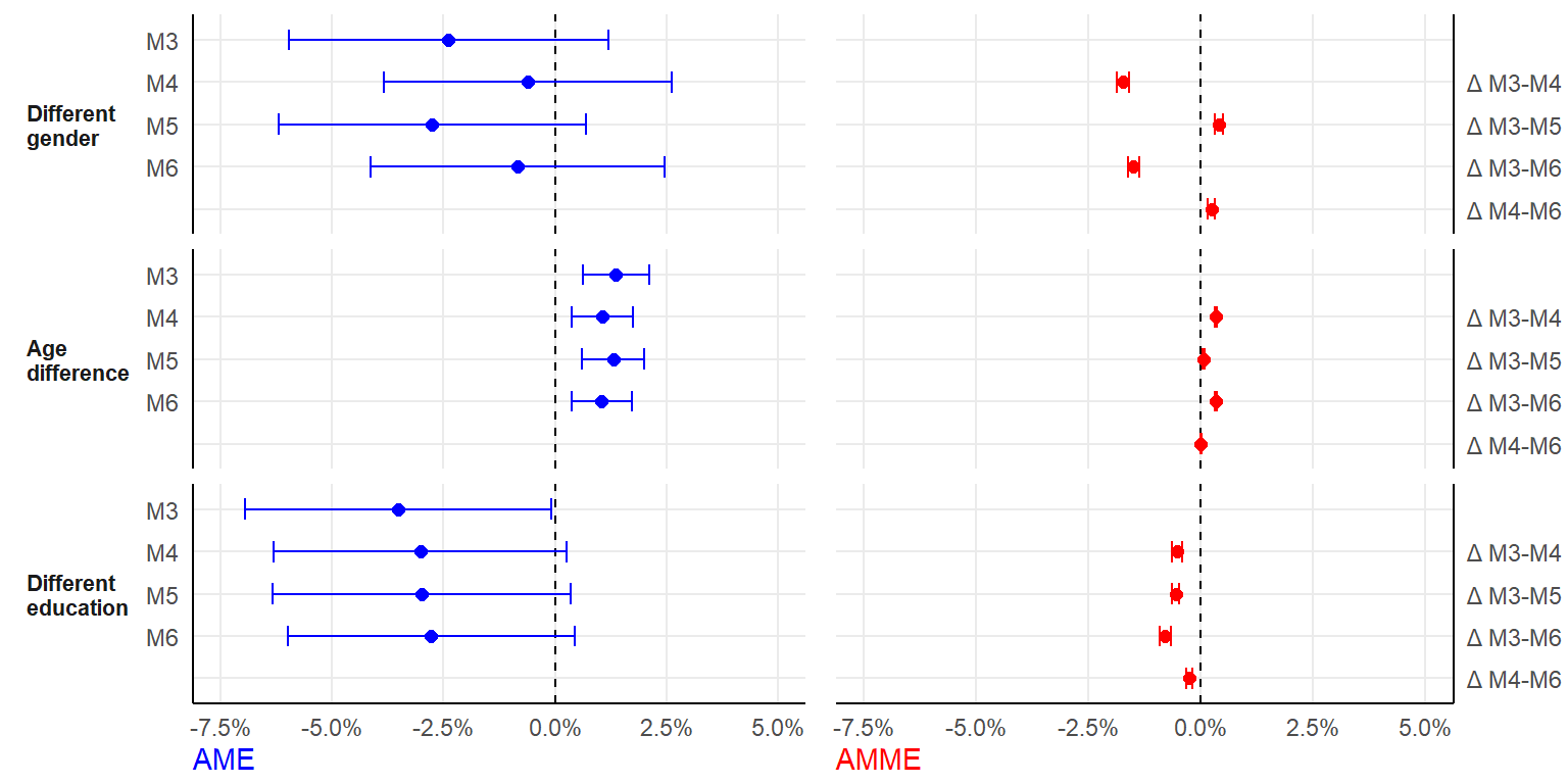
AME / AMIE
dissimilarity * tie type
gender <- data.frame(pred = "Different\ngender", model = c("Pooled", "best friends vs. confidants", "sports vs. confidants",
    "study vs. confidants"), ame = c(booL[[5]]$t0[1], rep(NA, 3)), ame_se = c(apply(booL[[5]]$t, 2, sd)[1],
    rep(NA, 3)), amie = c(NA, booL[[5]]$t0[2:4]), amie_se = c(NA, apply(booL[[5]]$t, 2, sd)[2:4]))

age <- data.frame(pred = "Age\ndifference", model = c("Pooled", "best friends vs. confidants", "sports vs. confidants",
    "study vs. confidants"), ame = c(booL[[5]]$t0[5], rep(NA, 3)), ame_se = c(apply(booL[[5]]$t, 2, sd)[5],
    rep(NA, 3)), amie = c(NA, booL[[5]]$t0[6:8]), amie_se = c(NA, apply(booL[[5]]$t, 2, sd)[6:8]))

educ <- data.frame(pred = "Different\neducation", model = c("Pooled", "best friends vs. confidants",
    "sports vs. confidants", "study vs. confidants"), ame = c(booL[[5]]$t0[9], rep(NA, 3)), ame_se = c(apply(booL[[5]]$t,
    2, sd)[9], rep(NA, 3)), amie = c(NA, booL[[5]]$t0[10:12]), amie_se = c(NA, apply(booL[[5]]$t, 2,
    sd)[10:12]))

plotdata <- rbind(gender, age, educ)

# variables to class factor, reorder:
plotdata$pred <- factor(plotdata$pred, levels = c("Different\ngender", "Age\ndifference", "Different\neducation"))
plotdata$model <- factor(plotdata$model, levels = rev(c("Pooled", "best friends vs. confidants", "sports vs. confidants",
    "study vs. confidants")))
plotdata <- plotdata[order(plotdata$pred), ]
row.names(plotdata) <- 1:nrow(plotdata)
fshowdf(plotdata, digits = 4)| pred | model | ame | ame_se | amie | amie_se |
|---|---|---|---|---|---|
| Different gender | Pooled | -0.0035 | 0.0170 | NA | NA |
| Different gender | best friends vs. confidants | NA | NA | 0.1502 | 0.0292 |
| Different gender | sports vs. confidants | NA | NA | 0.0826 | 0.0359 |
| Different gender | study vs. confidants | NA | NA | 0.1044 | 0.0350 |
| Age difference | Pooled | 0.0113 | 0.0035 | NA | NA |
| Age difference | best friends vs. confidants | NA | NA | 0.0098 | 0.0063 |
| Age difference | sports vs. confidants | NA | NA | -0.0226 | 0.0074 |
| Age difference | study vs. confidants | NA | NA | -0.0116 | 0.0080 |
| Different education | Pooled | -0.0214 | 0.0166 | NA | NA |
| Different education | best friends vs. confidants | NA | NA | -0.0083 | 0.0285 |
| Different education | sports vs. confidants | NA | NA | -0.0910 | 0.0349 |
| Different education | study vs. confidants | NA | NA | -0.0265 | 0.0383 |
#plot 1: AMEs
plot1 <- ggplot(plotdata, aes(x = ame, y = model, fill = pred)) +
  geom_vline(xintercept = 0, linetype = "dashed") + #vertical line at 0
  geom_point(size = 2, color = "blue") + #point indicating observed AME
  #geom_point(aes(x = ame_b, y = model, fill = pred), size = 3, shape = 4) + #cross indicating average bootstrap AME estimate
  geom_errorbar(aes(xmin = ame - 1.96*ame_se, xmax = ame + 1.96*ame_se), color="blue", width=.5) + #error bars for 95% CI
  facet_grid(pred ~., switch = "y", scales = "free_y", space = "free_y") + #arrange facets by dissimilarity type
  labs(x = "AME") + #rename x-axis name
  scale_x_continuous(labels = scales::percent, limits = c(-0.1, 0.1)) + #x-axis to %-point, and set range
  theme( #customize theme
    axis.title.y = element_blank(),
    axis.title.x = element_text(color = "blue"),
    strip.text.y.left = element_text(angle = 0),
    legend.position = "none",
    strip.background = element_blank(),
    strip.placement = "outside",
    strip.text.x = element_text(face = "bold"),
    axis.line = element_line()) +
  ggh4x::facetted_pos_scales(y = list( #customize y axis per facet..
  pred == "Different\ngender" ~ scale_y_discrete(labels = c( "", "", "", "M7")),
  pred == "Different\neducation" ~ scale_y_discrete(labels = c( "", "", "", "M7")),
  pred == "Age\ndifference" ~ scale_y_discrete(labels = c( "", "", "", "M7"))))


#plot 2: AMIEs
plot2 <- ggplot(plotdata, aes(x = amie, y = model, fill = pred)) +
  geom_vline(xintercept = 0, linetype = "dashed") +
  geom_point(size = 2, color = "orange") +
  geom_errorbar(aes(xmin = amie - 1.96*amie_se, xmax = amie + 1.96*amie_se), color="orange", width=.5) +
  facet_grid(pred ~., switch = "y", scales = "free_y", space = "free_y") +
  labs(x = "AMIE") +
  scale_x_continuous(labels = scales::percent, limits = c(-.25,.25)) + #x-axis to %-point, and set range
  theme(axis.title.y = element_blank(),
        axis.title.x = element_text(color = "orange"),
        legend.position = "none",
        strip.background = element_blank(),
        strip.placement = "outside",
        strip.text.x = element_text(face = "bold"),
        axis.line = element_line()) +
  scale_y_discrete(labels = c("study vs. confidant", "sports vs. confidant", "best friend vs. confidant", ""),
                   position = "right") +
  theme(strip.text = element_blank())

(figure <- ggarrange(plot1, plot2, ncol=2, align="hv", widths = c(1,1.2)))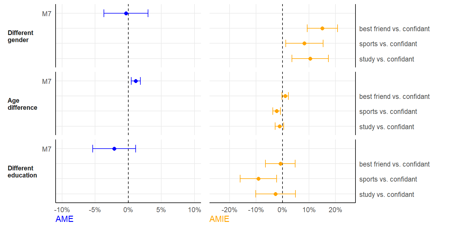
embeddedness * tie type
close <- data.frame(pred = "Emotional\ncloseness", model = c("Pooled", "best friends vs. confidants",
    "sports vs. confidants", "study vs. confidants"), ame = c(booL[[6]]$t0[1], rep(NA, 3)), ame_se = c(apply(booL[[6]]$t,
    2, sd)[1], rep(NA, 3)), amie = c(NA, booL[[6]]$t0[2:4]), amie_se = c(NA, apply(booL[[6]]$t, 2, sd)[2:4]))

multi <- data.frame(pred = "Relational\nmultiplexity", model = c("Pooled", "best friends vs. confidants",
    "sports vs. confidants", "study vs. confidants"), ame = c(booL[[6]]$t0[5], rep(NA, 3)), ame_se = c(apply(booL[[6]]$t,
    2, sd)[5], rep(NA, 3)), amie = c(NA, booL[[6]]$t0[6:8]), amie_se = c(NA, apply(booL[[6]]$t, 2, sd)[6:8]))

strf <- data.frame(pred = "Structural\nembedded-\nness\nfocal layer", model = c("Pooled", "best friends vs. confidants",
    "sports vs. confidants", "study vs. confidants"), ame = c(booL[[6]]$t0[9], rep(NA, 3)), ame_se = c(apply(booL[[6]]$t,
    2, sd)[9], rep(NA, 3)), amie = c(NA, booL[[6]]$t0[10:12]), amie_se = c(NA, apply(booL[[6]]$t, 2,
    sd)[10:12]))

stro <- data.frame(pred = "Structural\nembedded-\nness\nother layers", model = c("Pooled", "best friends vs. confidants",
    "sports vs. confidants", "study vs. confidants"), ame = c(booL[[6]]$t0[13], rep(NA, 3)), ame_se = c(apply(booL[[6]]$t,
    2, sd)[13], rep(NA, 3)), amie = c(NA, booL[[6]]$t0[14:16]), amie_se = c(NA, apply(booL[[6]]$t, 2,
    sd)[14:16]))

plotdata <- rbind(close, multi, strf, stro)

# variables to class factor, reorder:
plotdata$pred <- factor(plotdata$pred, levels = c("Emotional\ncloseness", "Relational\nmultiplexity",
    "Structural\nembedded-\nness\nfocal layer", "Structural\nembedded-\nness\nother layers"))

plotdata$model <- factor(plotdata$model, levels = rev(c("Pooled", "best friends vs. confidants", "sports vs. confidants",
    "study vs. confidants")))
plotdata <- plotdata[order(plotdata$pred), ]
row.names(plotdata) <- 1:nrow(plotdata)
fshowdf(plotdata, digits = 4)| pred | model | ame | ame_se | amie | amie_se |
|---|---|---|---|---|---|
| Emotional closeness | Pooled | -0.1425 | 0.0088 | NA | NA |
| Emotional closeness | best friends vs. confidants | NA | NA | 0.0552 | 0.0171 |
| Emotional closeness | sports vs. confidants | NA | NA | 0.0938 | 0.0234 |
| Emotional closeness | study vs. confidants | NA | NA | 0.1254 | 0.0236 |
| Relational multiplexity | Pooled | -0.0449 | 0.0093 | NA | NA |
| Relational multiplexity | best friends vs. confidants | NA | NA | 0.0411 | 0.0198 |
| Relational multiplexity | sports vs. confidants | NA | NA | 0.0995 | 0.0248 |
| Relational multiplexity | study vs. confidants | NA | NA | 0.0769 | 0.0239 |
| Structural embedded- ness focal layer | Pooled | -0.0551 | 0.0157 | NA | NA |
| Structural embedded- ness focal layer | best friends vs. confidants | NA | NA | 0.0279 | 0.0438 |
| Structural embedded- ness focal layer | sports vs. confidants | NA | NA | -0.0277 | 0.0514 |
| Structural embedded- ness focal layer | study vs. confidants | NA | NA | -0.1560 | 0.0482 |
| Structural embedded- ness other layers | Pooled | 0.0092 | 0.0465 | NA | NA |
| Structural embedded- ness other layers | best friends vs. confidants | NA | NA | 0.0279 | 0.0438 |
| Structural embedded- ness other layers | sports vs. confidants | NA | NA | -0.0271 | 0.0508 |
| Structural embedded- ness other layers | study vs. confidants | NA | NA | -0.1464 | 0.0462 |
#plot 1: AMEs
plot1 <- ggplot(plotdata, aes(x = ame, y = model, fill = pred)) +
  geom_vline(xintercept = 0, linetype = "dashed") + #vertical line at 0
  geom_point(size = 2, color = "blue") + #point indicating observed AME
  #geom_point(aes(x = ame_b, y = model, fill = pred), size = 3, shape = 4) + #cross indicating average bootstrap AME estimate
  geom_errorbar(aes(xmin = ame - 1.96*ame_se, xmax = ame + 1.96*ame_se), color="blue", width=.5) + #error bars for 95% CI
  facet_grid(pred ~., switch = "y", scales = "free_y", space = "free_y") + #arrange facets by dissimilarity type
  labs(x = "AME") + #rename x-axis name
 scale_x_continuous(labels = scales::percent, limits = c(-0.2, 0.15)) + #x-axis to %-point, and set range
  theme( #customize theme
    axis.title.y = element_blank(),
    axis.title.x = element_text(color = "blue"),
    strip.text.y.left = element_text(angle = 0),
    legend.position = "none",
    strip.background = element_blank(),
    strip.placement = "outside",
    strip.text.x = element_text(face = "bold"),
    axis.line = element_line()) +
  ggh4x::facetted_pos_scales(y = list( #customize y axis per facet..
  pred == "Emotional\ncloseness" ~ scale_y_discrete(labels = c( "", "", "", "M8")),
  pred == "Relational\nmultiplexity" ~ scale_y_discrete(labels = c( "", "", "", "M8")),
  pred == "Structural\nembedded-\nness\nfocal layer" ~ scale_y_discrete(labels = c( "", "", "", "M8")),
  pred == "Structural\nembedded-\nness\nother layers" ~ scale_y_discrete(labels = c( "", "", "", "M8"))
  ))


#plot 2: AMIEs
plot2 <- ggplot(plotdata, aes(x = amie, y = model, fill = pred)) +
  geom_vline(xintercept = 0, linetype = "dashed") +
  geom_point(size = 2, color = "orange") +
  geom_errorbar(aes(xmin = amie - 1.96*amie_se, xmax = amie + 1.96*amie_se), color="orange", width=.5) +
  facet_grid(pred ~., switch = "y", scales = "free_y", space = "free_y") +
  labs(x = "AMIE") +
  scale_x_continuous(labels = scales::percent, limits = c(-.3,.25)) + #x-axis to %-point, and set range
  theme(axis.title.y = element_blank(),
        axis.title.x = element_text(color = "orange"),
        legend.position = "none",
        strip.background = element_blank(),
        strip.placement = "outside",
        strip.text.x = element_text(face = "bold"),
        axis.line = element_line()) +
  scale_y_discrete(labels = c("study vs. confidant", "sports vs. confidant", "best friend vs. confidant", ""),
                   position = "right") +
  theme(strip.text = element_blank())


(figure <- ggarrange(plot1, plot2, ncol=2, align="hv", widths = c(1,1.2)))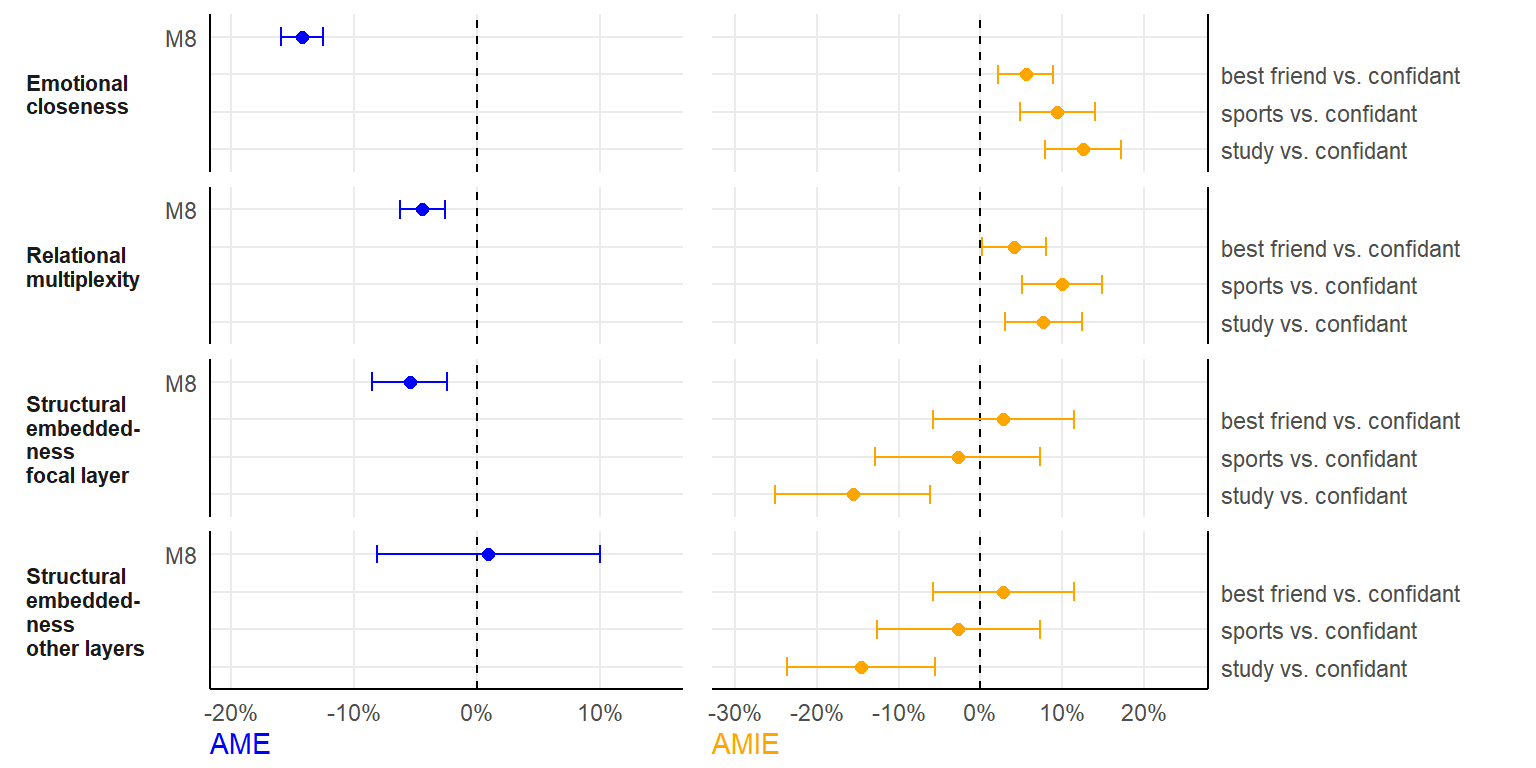
separate analyses by tie type
AMIEs provide a clear causal interpretation (i.e., how an AME changes when comparing a specific type of tie, when compared to confidants), but they lack a clear descriptive interpretation, regarding the significance and valence of AMEs across relational roles. To enhance our interpretation of AMIEs, we will compute AMEs (and AMMEs) for each specific network layer. This enables us to:
- assess the sign and significance of AMEs per relational role
- test mediation effects (AMMEs) per relational role
confidants
1. create new datasets
# dissimilarity
dfconfidantgender1 <- dfconfidantgender0 <- dfconfidant
dfconfidantageplus <- dfconfidantagemin <- dfconfidant
dfconfidanteduc1 <- dfconfidanteduc0 <- dfconfidant

dfconfidantgender1$different_gender <- 1
dfconfidantgender0$different_gender <- 0
dfconfidanteduc1$different_educ <- 1
dfconfidanteduc0$different_educ <- 0

# define small step for continuous variable
s <- 0.001
dfconfidantageplus$dif_age <- dfconfidant$dif_age + s
dfconfidantagemin$dif_age <- dfconfidant$dif_age - s

# embeddedness
dfconfidantcloseplus <- dfconfidantclosemin <- dfconfidant
dfconfidantcloseplus$closeness.t <- dfconfidant$closeness.t + s
dfconfidantclosemin$closeness.t <- dfconfidant$closeness.t - s

dfconfidantmultiplus <- dfconfidantmultimin <- dfconfidant
dfconfidantmultiplus$multiplex <- dfconfidant$multiplex + s
dfconfidantmultimin$multiplex <- dfconfidant$multiplex - s

dfconfidantfembedplus <- dfconfidantfembedmin <- dfconfidant
dfconfidantfembedplus$embed <- dfconfidant$embed + s
dfconfidantfembedmin$embed <- dfconfidant$embed - s

dfconfidantoembedplus <- dfconfidantoembedmin <- dfconfidant
dfconfidantoembedplus$embed.ext <- dfconfidant$embed.ext + s
dfconfidantoembedmin$embed.ext <- dfconfidant$embed.ext - s
2. get models
m1 <- ansconfidant[[2]]  #base
m2 <- ansconfidant[[3]]  #+mediator 1 (relational embeddedness)
m3 <- ansconfidant[[4]]  #+mediator 2 (structural embeddedness)
m4 <- ansconfidant[[5]]  #+both mediators
3. create fpred() functions
# 1. AMEs dissimilarities base model
fpred1 <- function(m1) {
    me_gender <- lme4:::predict.merMod(m1, type = "response", re.form = NULL, newdata = dfconfidantgender1) -
        lme4:::predict.merMod(m1, type = "response", re.form = NULL, newdata = dfconfidantgender0)
    ame_gender <- mean(me_gender)

    me_age <- (lme4:::predict.merMod(m1, type = "response", re.form = NULL, newdata = dfconfidantageplus) -
        lme4:::predict.merMod(m1, type = "response", re.form = NULL, newdata = dfconfidantagemin))/(2 *
        s)
    ame_age <- mean(me_age)

    me_educ <- lme4:::predict.merMod(m1, type = "response", re.form = NULL, newdata = dfconfidanteduc1) -
        lme4:::predict.merMod(m1, type = "response", re.form = NULL, newdata = dfconfidanteduc0)
    ame_educ <- mean(me_educ)

    c(ame_gender, ame_age, ame_educ)
}

# 2. after controlling for relational embeddedness
fpred2 <- function(m2) {
    me_gender <- lme4:::predict.merMod(m2, type = "response", re.form = NULL, newdata = dfconfidantgender1) -
        lme4:::predict.merMod(m2, type = "response", re.form = NULL, newdata = dfconfidantgender0)
    ame_gender <- mean(me_gender)

    me_age <- (lme4:::predict.merMod(m2, type = "response", re.form = NULL, newdata = dfconfidantageplus) -
        lme4:::predict.merMod(m2, type = "response", re.form = NULL, newdata = dfconfidantagemin))/(2 *
        s)
    ame_age <- mean(me_age)

    me_educ <- lme4:::predict.merMod(m2, type = "response", re.form = NULL, newdata = dfconfidanteduc1) -
        lme4:::predict.merMod(m2, type = "response", re.form = NULL, newdata = dfconfidanteduc0)
    ame_educ <- mean(me_educ)

    c(ame_gender, ame_age, ame_educ)
}

# 3. after controlling for structural embeddedness
fpred3 <- function(m3) {
    me_gender <- lme4:::predict.merMod(m3, type = "response", re.form = NULL, newdata = dfconfidantgender1) -
        lme4:::predict.merMod(m3, type = "response", re.form = NULL, newdata = dfconfidantgender0)
    ame_gender <- mean(me_gender)

    me_age <- (lme4:::predict.merMod(m3, type = "response", re.form = NULL, newdata = dfconfidantageplus) -
        lme4:::predict.merMod(m3, type = "response", re.form = NULL, newdata = dfconfidantagemin))/(2 *
        s)
    ame_age <- mean(me_age)

    me_educ <- lme4:::predict.merMod(m3, type = "response", re.form = NULL, newdata = dfconfidanteduc1) -
        lme4:::predict.merMod(m3, type = "response", re.form = NULL, newdata = dfconfidanteduc0)
    ame_educ <- mean(me_educ)

    c(ame_gender, ame_age, ame_educ)
}

# 4. after controlling for both mediators
fpred4 <- function(m4) {
    me_gender <- lme4:::predict.merMod(m4, type = "response", re.form = NULL, newdata = dfconfidantgender1) -
        lme4:::predict.merMod(m4, type = "response", re.form = NULL, newdata = dfconfidantgender0)
    ame_gender <- mean(me_gender)

    me_age <- (lme4:::predict.merMod(m4, type = "response", re.form = NULL, newdata = dfconfidantageplus) -
        lme4:::predict.merMod(m4, type = "response", re.form = NULL, newdata = dfconfidantagemin))/(2 *
        s)
    ame_age <- mean(me_age)

    me_educ <- lme4:::predict.merMod(m4, type = "response", re.form = NULL, newdata = dfconfidanteduc1) -
        lme4:::predict.merMod(m4, type = "response", re.form = NULL, newdata = dfconfidanteduc0)
    ame_educ <- mean(me_educ)

    # also AMEs of embeddedness
    me_close <- (lme4:::predict.merMod(m4, type = "response", re.form = NULL, newdata = dfconfidantcloseplus) -
        lme4:::predict.merMod(m4, type = "response", re.form = NULL, newdata = dfconfidantclosemin))/(2 *
        s)
    ame_close <- mean(me_close)
    summary(m4)

    me_multi <- (lme4:::predict.merMod(m4, type = "response", re.form = NULL, newdata = dfconfidantmultiplus) -
        lme4:::predict.merMod(m4, type = "response", re.form = NULL, newdata = dfconfidantmultimin))/(2 *
        s)
    ame_multi <- mean(me_multi)

    me_fembed <- (lme4:::predict.merMod(m4, type = "response", re.form = NULL, newdata = dfconfidantfembedplus) -
        lme4:::predict.merMod(m4, type = "response", re.form = NULL, newdata = dfconfidantfembedmin))/(2 *
        s)
    ame_fembed <- mean(me_fembed)

    me_oembed <- (lme4:::predict.merMod(m4, type = "response", re.form = NULL, newdata = dfconfidantoembedplus) -
        lme4:::predict.merMod(m4, type = "response", re.form = NULL, newdata = dfconfidantoembedmin))/(2 *
        s)
    ame_oembed <- mean(me_oembed)

    c(ame_gender, ame_age, ame_educ, ame_close, ame_multi, ame_fembed, ame_oembed)
}

# fpred1(m1) fpred2(m2) fpred3(m3) fpred4(m4)
4. bootstrap AMEs
seed <- 2425323
nIter <- 500

nCore <- parallel::detectCores()
mycl <- makeCluster(rep("localhost", nCore))
clusterEvalQ(mycl, library(lme4))
clusterExport(mycl, varlist = c("m1", "m2", "m3", "m4", "s", "seed", "dfconfidantgender1", "dfconfidantgender0",
    "dfconfidantageplus", "dfconfidantagemin", "dfconfidanteduc1", "dfconfidanteduc0", "dfconfidantcloseplus",
    "dfconfidantclosemin", "dfconfidantmultiplus", "dfconfidantmultimin", "dfconfidantfembedplus", "dfconfidantfembedmin",
    "dfconfidantoembedplus", "dfconfidantoembedmin"))

system.time(boo_m1 <- bootMer(m1, fpred1, nsim = nIter, parallel = "snow", ncpus = nCore, cl = mycl,
    seed = seed))
system.time(boo_m2 <- bootMer(m2, fpred2, nsim = nIter, parallel = "snow", ncpus = nCore, cl = mycl,
    seed = seed))
system.time(boo_m3 <- bootMer(m3, fpred3, nsim = nIter, parallel = "snow", ncpus = nCore, cl = mycl,
    seed = seed))
system.time(boo_m4 <- bootMer(m4, fpred4, nsim = nIter, parallel = "snow", ncpus = nCore, cl = mycl,
    seed = seed))

booL <- list(boo_m1, boo_m2, boo_m3, boo_m4)
save(booL, file = "./results/boot_confidants.Rda")
stopCluster(mycl)
5. construct plot dataset
nIter = 500
load("./results/boot_confidants.rda")

# AMEs dissimilarities
plotdata <- data.frame(pred = rep(c("Different\ngender", "Age\ndifference", "Different\neducation"),
    4), model = rep(c("M3", "M4", "M5", "M6"), each = 3), ame = c(booL[[1]]$t0, booL[[2]]$t0, booL[[3]]$t0,
    booL[[4]]$t0[1:3]), ame_se = c(apply(booL[[1]]$t, 2, sd), apply(booL[[2]]$t, 2, sd), apply(booL[[3]]$t,
    2, sd), apply(booL[[4]]$t, 2, sd)[1:3]))

# AMMEs
plotdata$amme <- NA
plotdata$amme_se <- NA

for (i in c(1:3)) {
    # for dissimilarity ground for extended model get AMEs of dissimilarity i of baseline model
    for (j in c(2:4)) {
        ame_i_base <- booL[[1]]$t[, i]
        # get AMEs of dissimilarity i of extended model j
        ame_i_modelj <- booL[[j]]$t[, i]
        # calculate cross-model AME difference per bootstrap iteration
        cm_ame_difs <- ame_i_base - ame_i_modelj
        # calculate average marginal mediation effect by taking the average
        plotdata$amme[plotdata$pred == unique(plotdata$pred)[i] & plotdata$model == unique(plotdata$model)[j]] <- mean(cm_ame_difs)
        # and SE
        plotdata$amme_se[plotdata$pred == unique(plotdata$pred)[i] & plotdata$model == unique(plotdata$model)[j]] <- sd(cm_ame_difs)/sqrt(nIter)
    }
}

plotdata2 <- data.frame(pred = c("Different\ngender", "Age\ndifference", "Different\neducation"), model = "M4-M6",
    ame = NA, ame_se = NA, amme = NA, amme_se = NA)

for (i in c(1:3)) {
    # get AMEs of dissimilarity i of model 2 (including relational embeddedness only)
    ame_i_base <- booL[[2]]$t[, i]
    # get AME of dissimilarity i of extended model 4 (adding also structural embeddedness)
    ame_i_modelj <- booL[[4]]$t[, i]
    # calculate cross-model AME difference
    cm_ame_difs <- ame_i_base - ame_i_modelj
    # calcualte average marginal mediation
    plotdata2$amme[plotdata2$pred == unique(plotdata2$pred)[i]] <- mean(cm_ame_difs)
    # and SE
    plotdata2$amme_se[plotdata2$pred == unique(plotdata2$pred)[i]] <- sd(cm_ame_difs)/sqrt(nIter)
}

# AME embeddedness
plotdata3 <- data.frame(pred = c("Emotional\ncloseness", "Relational\nmultiplexity", "Str. embed.\nfocal layer",
    "Str. embed.\nother layers"), model = "M6", ame = booL[[4]]$t0[4:7], ame_se = apply(booL[[4]]$t,
    2, sd)[4:7])

bind_rows(plotdata, plotdata2, plotdata3) -> plotdata

plotdata$pred <- factor(plotdata$pred, levels = c("Different\ngender", "Age\ndifference", "Different\neducation",
    "Emotional\ncloseness", "Relational\nmultiplexity", "Str. embed.\nfocal layer", "Str. embed.\nother layers"))
plotdata$model <- factor(plotdata$model, levels = rev(c("M2", "M4", "M5", "M6", "M4-M6")))
plotdata <- plotdata[order(plotdata$pred), ]
row.names(plotdata) <- 1:nrow(plotdata)
6. result
#plot 1: AMEs
plot1 <- ggplot(plotdata, aes(x = ame, y = model, fill = pred)) +
  geom_vline(xintercept = 0, linetype = "dashed") + #vertical line at 0
  geom_point(size = 2, color = "blue") + #point indicating observed AME
  #geom_point(aes(x = ame_b, y = model, fill = pred), size = 3, shape = 4) + #cross indicating average bootstrap AME estimate
  geom_errorbar(aes(xmin = ame - 1.96*ame_se, xmax = ame + 1.96*ame_se), color="blue", width=.5) + #error bars for 95% CI
  facet_grid(pred ~., switch = "y", scales = "free_y", space = "free_y") + #arrange facets by dissimilarity type
  labs(x = "AME") + #rename x-axis name
  scale_x_continuous(labels = scales::percent, limits = c(-0.25, 0.30)) + #x-axis to %-point, and set range
  theme( #customize theme
    axis.title.y = element_blank(),
    axis.title.x = element_text(color = "blue"),
    strip.text.y.left = element_text(angle = 0),
    legend.position = "none",
    strip.background = element_blank(),
    strip.placement = "outside",
    strip.text.x = element_text(face = "bold"),
    axis.line = element_line()) +
    ggh4x::facetted_pos_scales(y = list( #customize y axis per facet..
      pred == "Different\ngender" ~ scale_y_discrete(labels = c("", "M6", "M5", "M4", "M3")),
      pred == "Age\ndifference" ~ scale_y_discrete(labels = c("", "M6", "M5", "M4", "M3")),
      pred == "Different\neducation" ~ scale_y_discrete(labels = c("", "M6", "M5", "M4", "M3")),
      pred == "Emotional\ncloseness" ~ scale_y_discrete(labels = "M6"),
      pred == "Relational\nmultiplexity" ~ scale_y_discrete(labels = "M6"),
      pred == "Str. embed.\nfocal layer" ~ scale_y_discrete(labels = "M6"),
      pred == "Str. embed.\nother layers" ~ scale_y_discrete(labels = "M6")
      ))

plot2 <- ggplot(plotdata, aes(x = amme, y = model, fill = pred)) +
  geom_vline(xintercept = 0, linetype = "dashed") +
  geom_point(size = 2, color = "red") +
  geom_errorbar(aes(xmin = amme - 1.96*amme_se, xmax = amme + 1.96*amme_se), color="red", width=.5) +
  facet_grid(pred ~., switch = "y", scales = "free_y", space = "free_y") +
  labs(x = "AMME") +
  scale_x_continuous(labels = scales::percent, limits = c(-0.05, 0.05)) +
  theme(axis.title.y = element_blank(),
        axis.title.x = element_text(color = "red"),
        legend.position = "none",
        strip.background = element_blank(),
        strip.placement = "outside",
        strip.text.x = element_text(face = "bold"),
        axis.line = element_line()) +
  ggh4x::facetted_pos_scales(y = list( #customize y axis per facet..
    pred == "Different\ngender" ~ scale_y_discrete(labels = c("Δ M4-M6", "Δ M3-M6", "Δ M3-M5", "Δ M3-M4", ""), position = "right"),
    pred == "Age\ndifference" ~ scale_y_discrete(labels = c("Δ M4-M6", "Δ M3-M6", "Δ M3-M5", "Δ M3-M4", ""), position = "right"),
    pred == "Different\neducation" ~ scale_y_discrete(labels = c("Δ M4-M6", "Δ M3-M6", "Δ M3-M5", "Δ M3-M4", ""), position = "right"),
    pred == "Emotional\ncloseness" ~ scale_y_discrete(labels = NULL, position = "right"),
    pred == "Relational\nmultiplexity" ~ scale_y_discrete(labels = NULL, position = "right"),
    pred == "Str. embed.\nfocal layer" ~  scale_y_discrete(labels = NULL, position = "right"),
    pred == "Str. embed.\nother layers" ~ scale_y_discrete(labels = NULL, position = "right"))) +
  theme(strip.text = element_blank())

#combine plots
#?ggarrange
fshowdf(plotdata,digits=3)| pred | model | ame | ame_se | amme | amme_se |
|---|---|---|---|---|---|
| Different gender | NA | -0.073 | 0.028 | NA | NA |
| Different gender | M4 | -0.071 | 0.028 | -0.001 | 0.001 |
| Different gender | M5 | -0.089 | 0.028 | 0.017 | 0.001 |
| Different gender | M6 | -0.071 | 0.028 | -0.001 | 0.001 |
| Different gender | M4-M6 | NA | NA | 0.000 | 0.000 |
| Age difference | NA | 0.022 | 0.005 | NA | NA |
| Age difference | M4 | 0.010 | 0.005 | 0.012 | 0.000 |
| Age difference | M5 | 0.021 | 0.005 | 0.001 | 0.000 |
| Age difference | M6 | 0.010 | 0.005 | 0.012 | 0.000 |
| Age difference | M4-M6 | NA | NA | 0.000 | 0.000 |
| Different education | NA | -0.018 | 0.027 | NA | NA |
| Different education | M4 | -0.014 | 0.026 | -0.004 | 0.001 |
| Different education | M5 | -0.016 | 0.027 | -0.003 | 0.001 |
| Different education | M6 | -0.014 | 0.026 | -0.005 | 0.001 |
| Different education | M4-M6 | NA | NA | -0.001 | 0.000 |
| Emotional closeness | M6 | -0.179 | 0.016 | NA | NA |
| Relational multiplexity | M6 | -0.103 | 0.016 | NA | NA |
| Str. embed. focal layer | M6 | -0.016 | 0.037 | NA | NA |
| Str. embed. other layers | M6 | 0.021 | 0.068 | NA | NA |
figure <- ggarrange(plot1, plot2, ncol=2, widths=c(1.1, 1))
(figure <- annotate_figure(figure, top = text_grob("Confidants", color = "black", face = "bold", size = 14)))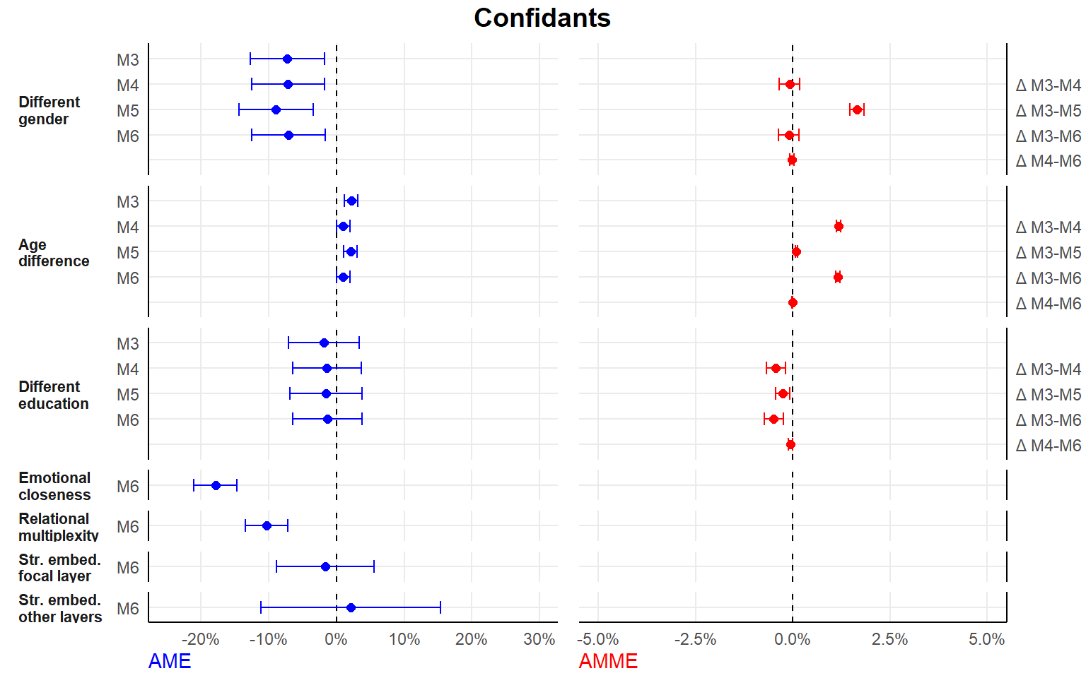
best friends
1. create new datasets
# dissimilarity
dffriendgender1 <- dffriendgender0 <- dffriend
dffriendageplus <- dffriendagemin <- dffriend
dffriendeduc1 <- dffriendeduc0 <- dffriend

dffriendgender1$different_gender <- 1
dffriendgender0$different_gender <- 0
dffriendeduc1$different_educ <- 1
dffriendeduc0$different_educ <- 0

# define small step for continuous variable
s <- 0.001
dffriendageplus$dif_age <- dffriend$dif_age + s
dffriendagemin$dif_age <- dffriend$dif_age - s

# embeddedness
dffriendcloseplus <- dffriendclosemin <- dffriend
dffriendcloseplus$closeness.t <- dffriend$closeness.t + s
dffriendclosemin$closeness.t <- dffriend$closeness.t - s

dffriendmultiplus <- dffriendmultimin <- dffriend
dffriendmultiplus$multiplex <- dffriend$multiplex + s
dffriendmultimin$multiplex <- dffriend$multiplex - s

dffriendfembedplus <- dffriendfembedmin <- dffriend
dffriendfembedplus$embed <- dffriend$embed + s
dffriendfembedmin$embed <- dffriend$embed - s

dffriendoembedplus <- dffriendoembedmin <- dffriend
dffriendoembedplus$embed.ext <- dffriend$embed.ext + s
dffriendoembedmin$embed.ext <- dffriend$embed.ext - s
2. get models
m1 <- ansfriend[[2]]  #base
m2 <- ansfriend[[3]]  #+mediator 1 (relational embeddedness)
m3 <- ansfriend[[4]]  #+mediator 2 (structural embeddedness)
m4 <- ansfriend[[5]]  #+both mediators
3. create fpred() functions
# 1. AMEs dissimilarities base model
fpred1 <- function(m1) {
    me_gender <- lme4:::predict.merMod(m1, type = "response", re.form = NULL, newdata = dffriendgender1) -
        lme4:::predict.merMod(m1, type = "response", re.form = NULL, newdata = dffriendgender0)
    ame_gender <- mean(me_gender)

    me_age <- (lme4:::predict.merMod(m1, type = "response", re.form = NULL, newdata = dffriendageplus) -
        lme4:::predict.merMod(m1, type = "response", re.form = NULL, newdata = dffriendagemin))/(2 *
        s)
    ame_age <- mean(me_age)

    me_educ <- lme4:::predict.merMod(m1, type = "response", re.form = NULL, newdata = dffriendeduc1) -
        lme4:::predict.merMod(m1, type = "response", re.form = NULL, newdata = dffriendeduc0)
    ame_educ <- mean(me_educ)

    c(ame_gender, ame_age, ame_educ)
}

# 2. after controlling for relational embeddedness
fpred2 <- function(m2) {
    me_gender <- lme4:::predict.merMod(m2, type = "response", re.form = NULL, newdata = dffriendgender1) -
        lme4:::predict.merMod(m2, type = "response", re.form = NULL, newdata = dffriendgender0)
    ame_gender <- mean(me_gender)

    me_age <- (lme4:::predict.merMod(m2, type = "response", re.form = NULL, newdata = dffriendageplus) -
        lme4:::predict.merMod(m2, type = "response", re.form = NULL, newdata = dffriendagemin))/(2 *
        s)
    ame_age <- mean(me_age)

    me_educ <- lme4:::predict.merMod(m2, type = "response", re.form = NULL, newdata = dffriendeduc1) -
        lme4:::predict.merMod(m2, type = "response", re.form = NULL, newdata = dffriendeduc0)
    ame_educ <- mean(me_educ)

    c(ame_gender, ame_age, ame_educ)
}

# 3. after controlling for structural embeddedness
fpred3 <- function(m3) {
    me_gender <- lme4:::predict.merMod(m3, type = "response", re.form = NULL, newdata = dffriendgender1) -
        lme4:::predict.merMod(m3, type = "response", re.form = NULL, newdata = dffriendgender0)
    ame_gender <- mean(me_gender)

    me_age <- (lme4:::predict.merMod(m3, type = "response", re.form = NULL, newdata = dffriendageplus) -
        lme4:::predict.merMod(m3, type = "response", re.form = NULL, newdata = dffriendagemin))/(2 *
        s)
    ame_age <- mean(me_age)

    me_educ <- lme4:::predict.merMod(m3, type = "response", re.form = NULL, newdata = dffriendeduc1) -
        lme4:::predict.merMod(m3, type = "response", re.form = NULL, newdata = dffriendeduc0)
    ame_educ <- mean(me_educ)

    c(ame_gender, ame_age, ame_educ)
}

# 4. after controlling for both mediators
fpred4 <- function(m4) {
    me_gender <- lme4:::predict.merMod(m4, type = "response", re.form = NULL, newdata = dffriendgender1) -
        lme4:::predict.merMod(m4, type = "response", re.form = NULL, newdata = dffriendgender0)
    ame_gender <- mean(me_gender)

    me_age <- (lme4:::predict.merMod(m4, type = "response", re.form = NULL, newdata = dffriendageplus) -
        lme4:::predict.merMod(m4, type = "response", re.form = NULL, newdata = dffriendagemin))/(2 *
        s)
    ame_age <- mean(me_age)

    me_educ <- lme4:::predict.merMod(m4, type = "response", re.form = NULL, newdata = dffriendeduc1) -
        lme4:::predict.merMod(m4, type = "response", re.form = NULL, newdata = dffriendeduc0)
    ame_educ <- mean(me_educ)

    # also AMEs of embeddedness
    me_close <- (lme4:::predict.merMod(m4, type = "response", re.form = NULL, newdata = dffriendcloseplus) -
        lme4:::predict.merMod(m4, type = "response", re.form = NULL, newdata = dffriendclosemin))/(2 *
        s)
    ame_close <- mean(me_close)
    summary(m4)

    me_multi <- (lme4:::predict.merMod(m4, type = "response", re.form = NULL, newdata = dffriendmultiplus) -
        lme4:::predict.merMod(m4, type = "response", re.form = NULL, newdata = dffriendmultimin))/(2 *
        s)
    ame_multi <- mean(me_multi)

    me_fembed <- (lme4:::predict.merMod(m4, type = "response", re.form = NULL, newdata = dffriendfembedplus) -
        lme4:::predict.merMod(m4, type = "response", re.form = NULL, newdata = dffriendfembedmin))/(2 *
        s)
    ame_fembed <- mean(me_fembed)

    me_oembed <- (lme4:::predict.merMod(m4, type = "response", re.form = NULL, newdata = dffriendoembedplus) -
        lme4:::predict.merMod(m4, type = "response", re.form = NULL, newdata = dffriendoembedmin))/(2 *
        s)
    ame_oembed <- mean(me_oembed)

    c(ame_gender, ame_age, ame_educ, ame_close, ame_multi, ame_fembed, ame_oembed)
}

# fpred1(m1) fpred2(m2) fpred3(m3) fpred4(m4)
4. bootstrap AMEs
seed <- 2425323
nIter <- 500

nCore <- parallel::detectCores()
mycl <- makeCluster(rep("localhost", nCore))
clusterEvalQ(mycl, library(lme4))
clusterExport(mycl, varlist = c("m1", "m2", "m3", "m4", "s", "seed", "dffriendgender1", "dffriendgender0",
    "dffriendageplus", "dffriendagemin", "dffriendeduc1", "dffriendeduc0", "dffriendcloseplus", "dffriendclosemin",
    "dffriendmultiplus", "dffriendmultimin", "dffriendfembedplus", "dffriendfembedmin", "dffriendoembedplus",
    "dffriendoembedmin"))

system.time(boo_m1 <- bootMer(m1, fpred1, nsim = nIter, parallel = "snow", ncpus = nCore, cl = mycl,
    seed = seed))
system.time(boo_m2 <- bootMer(m2, fpred2, nsim = nIter, parallel = "snow", ncpus = nCore, cl = mycl,
    seed = seed))
system.time(boo_m3 <- bootMer(m3, fpred3, nsim = nIter, parallel = "snow", ncpus = nCore, cl = mycl,
    seed = seed))
system.time(boo_m4 <- bootMer(m4, fpred4, nsim = nIter, parallel = "snow", ncpus = nCore, cl = mycl,
    seed = seed))

booL <- list(boo_m1, boo_m2, boo_m3, boo_m4)
save(booL, file = "./results/boot_friends.Rda")
stopCluster(mycl)
5. construct plot dataset
nIter = 500
load("./results/boot_friends.rda")

# AMEs dissimilarities
plotdata <- data.frame(pred = rep(c("Different\ngender", "Age\ndifference", "Different\neducation"),
    4), model = rep(c("M3", "M4", "M5", "M6"), each = 3), ame = c(booL[[1]]$t0, booL[[2]]$t0, booL[[3]]$t0,
    booL[[4]]$t0[1:3]), ame_se = c(apply(booL[[1]]$t, 2, sd), apply(booL[[2]]$t, 2, sd), apply(booL[[3]]$t,
    2, sd), apply(booL[[4]]$t, 2, sd)[1:3]))

# AMMEs
plotdata$amme <- NA
plotdata$amme_se <- NA

for (i in c(1:3)) {
    # for dissimilarity ground for extended model get AMEs of dissimilarity i of baseline model
    for (j in c(2:4)) {
        ame_i_base <- booL[[1]]$t[, i]
        # get AMEs of dissimilarity i of extended model j
        ame_i_modelj <- booL[[j]]$t[, i]
        # calculate cross-model AME difference per bootstrap iteration
        cm_ame_difs <- ame_i_base - ame_i_modelj
        # calculate average marginal mediation effect by taking the average
        plotdata$amme[plotdata$pred == unique(plotdata$pred)[i] & plotdata$model == unique(plotdata$model)[j]] <- mean(cm_ame_difs)
        # and SE
        plotdata$amme_se[plotdata$pred == unique(plotdata$pred)[i] & plotdata$model == unique(plotdata$model)[j]] <- sd(cm_ame_difs)/sqrt(nIter)
    }
}

plotdata2 <- data.frame(pred = c("Different\ngender", "Age\ndifference", "Different\neducation"), model = "M4-M6",
    ame = NA, ame_se = NA, amme = NA, amme_se = NA)

for (i in c(1:3)) {
    # get AMEs of dissimilarity i of model 2 (including relational embeddedness only)
    ame_i_base <- booL[[2]]$t[, i]
    # get AME of dissimilarity i of extended model 4 (adding also structural embeddedness)
    ame_i_modelj <- booL[[4]]$t[, i]
    # calculate cross-model AME difference
    cm_ame_difs <- ame_i_base - ame_i_modelj
    # calcualte average marginal mediation
    plotdata2$amme[plotdata2$pred == unique(plotdata2$pred)[i]] <- mean(cm_ame_difs)
    # and SE
    plotdata2$amme_se[plotdata2$pred == unique(plotdata2$pred)[i]] <- sd(cm_ame_difs)/sqrt(nIter)
}

# AME embeddedness
plotdata3 <- data.frame(pred = c("Emotional\ncloseness", "Relational\nmultiplexity", "Str. embed.\nfocal layer",
    "Str. embed.\nother layers"), model = "M6", ame = booL[[4]]$t0[4:7], ame_se = apply(booL[[4]]$t,
    2, sd)[4:7])

bind_rows(plotdata, plotdata2, plotdata3) -> plotdata

plotdata$pred <- factor(plotdata$pred, levels = c("Different\ngender", "Age\ndifference", "Different\neducation",
    "Emotional\ncloseness", "Relational\nmultiplexity", "Str. embed.\nfocal layer", "Str. embed.\nother layers"))
plotdata$model <- factor(plotdata$model, levels = rev(c("M3", "M4", "M5", "M6", "M4-M6")))
plotdata <- plotdata[order(plotdata$pred), ]
row.names(plotdata) <- 1:nrow(plotdata)
6. result
#plot 1: AMEs
plot1 <- ggplot(plotdata, aes(x = ame, y = model, fill = pred)) +
  geom_vline(xintercept = 0, linetype = "dashed") + #vertical line at 0
  geom_point(size = 2, color = "blue") + #point indicating observed AME
  #geom_point(aes(x = ame_b, y = model, fill = pred), size = 3, shape = 4) + #cross indicating average bootstrap AME estimate
  geom_errorbar(aes(xmin = ame - 1.96*ame_se, xmax = ame + 1.96*ame_se), color="blue", width=.5) + #error bars for 95% CI
  facet_grid(pred ~., switch = "y", scales = "free_y", space = "free_y") + #arrange facets by dissimilarity type
  labs(x = "AME") + #rename x-axis name
  scale_x_continuous(labels = scales::percent, limits = c(-0.25, .30)) + #x-axis to %-point, and set range
  theme( #customize theme
    axis.title.y = element_blank(),
    axis.title.x = element_text(color = "blue"),
    strip.text.y.left = element_text(angle = 0),
    legend.position = "none",
    strip.background = element_blank(),
    strip.placement = "outside",
    strip.text.x = element_text(face = "bold"),
    axis.line = element_line()) +
    ggh4x::facetted_pos_scales(y = list( #customize y axis per facet..
      pred == "Different\ngender" ~ scale_y_discrete(labels = c("", "M6", "M5", "M4", "M3")),
      pred == "Age\ndifference" ~ scale_y_discrete(labels = c("", "M6", "M5", "M4", "M3")),
      pred == "Different\neducation" ~ scale_y_discrete(labels = c("", "M6", "M5", "M4", "M3")),
      pred == "Emotional\ncloseness" ~ scale_y_discrete(labels = "M6"),
      pred == "Relational\nmultiplexity" ~ scale_y_discrete(labels = "M6"),
      pred == "Str. embed.\nfocal layer" ~ scale_y_discrete(labels = "M6"),
      pred == "Str. embed.\nother layers" ~ scale_y_discrete(labels = "M6")
      ))

plot2 <- ggplot(plotdata, aes(x = amme, y = model, fill = pred)) +
  geom_vline(xintercept = 0, linetype = "dashed") +
  geom_point(size = 2, color = "red") +
  geom_errorbar(aes(xmin = amme - 1.96*amme_se, xmax = amme + 1.96*amme_se), color="red", width=.5) +
  facet_grid(pred ~., switch = "y", scales = "free_y", space = "free_y") +
  labs(x = "AMME") +
  scale_x_continuous(labels = scales::percent, limits = c(-0.05, 0.05)) +
  theme(axis.title.y = element_blank(),
        axis.title.x = element_text(color = "red"),
        legend.position = "none",
        strip.background = element_blank(),
        strip.placement = "outside",
        strip.text.x = element_text(face = "bold"),
        axis.line = element_line()) +
  ggh4x::facetted_pos_scales(y = list( #customize y axis per facet..
    pred == "Different\ngender" ~ scale_y_discrete(labels = c("Δ M4-M6", "Δ M3-M6", "Δ M3-M5", "Δ M3-M4", ""), position = "right"),
    pred == "Age\ndifference" ~ scale_y_discrete(labels = c("Δ M4-M6", "Δ M3-M6", "Δ M3-M5", "Δ M3-M4", ""), position = "right"),
    pred == "Different\neducation" ~ scale_y_discrete(labels = c("Δ M4-M6", "Δ M3-M6", "Δ M3-M5", "Δ M3-M4", ""), position = "right"),
    pred == "Emotional\ncloseness" ~ scale_y_discrete(labels = NULL, position = "right"),
    pred == "Relational\nmultiplexity" ~ scale_y_discrete(labels = NULL, position = "right"),
    pred == "Str. embed.\nfocal layer" ~  scale_y_discrete(labels = NULL, position = "right"),
    pred == "Str. embed.\nother layers" ~ scale_y_discrete(labels = NULL, position = "right"))) +
  theme(strip.text = element_blank())

#combine plots
#?ggarrange
fshowdf(plotdata, digits=3)| pred | model | ame | ame_se | amme | amme_se |
|---|---|---|---|---|---|
| Different gender | M3 | 0.002 | 0.026 | NA | NA |
| Different gender | M4 | 0.015 | 0.026 | -0.012 | 0.001 |
| Different gender | M5 | 0.008 | 0.026 | -0.003 | 0.001 |
| Different gender | M6 | 0.015 | 0.025 | -0.013 | 0.001 |
| Different gender | M4-M6 | NA | NA | -0.001 | 0.000 |
| Age difference | M3 | 0.016 | 0.005 | NA | NA |
| Age difference | M4 | 0.018 | 0.006 | -0.001 | 0.000 |
| Age difference | M5 | 0.017 | 0.005 | -0.001 | 0.000 |
| Age difference | M6 | 0.018 | 0.006 | -0.001 | 0.000 |
| Age difference | M4-M6 | NA | NA | 0.000 | 0.000 |
| Different education | M3 | 0.014 | 0.024 | NA | NA |
| Different education | M4 | 0.018 | 0.022 | -0.005 | 0.001 |
| Different education | M5 | 0.014 | 0.022 | 0.001 | 0.001 |
| Different education | M6 | 0.017 | 0.022 | -0.003 | 0.001 |
| Different education | M4-M6 | NA | NA | 0.001 | 0.000 |
| Emotional closeness | M6 | -0.132 | 0.013 | NA | NA |
| Relational multiplexity | M6 | -0.081 | 0.014 | NA | NA |
| Str. embed. focal layer | M6 | 0.024 | 0.027 | NA | NA |
| Str. embed. other layers | M6 | -0.098 | 0.072 | NA | NA |
figure <- ggarrange(plot1, plot2, ncol=2, widths=c(1.1, 1))
(figure <- annotate_figure(figure, top = text_grob("Best friends", color = "black", face = "bold", size = 14)))
sports partners
1. create new datasets
# dissimilarity
dfsportgender1 <- dfsportgender0 <- dfsport
dfsportageplus <- dfsportagemin <- dfsport
dfsporteduc1 <- dfsporteduc0 <- dfsport

dfsportgender1$different_gender <- 1
dfsportgender0$different_gender <- 0
dfsporteduc1$different_educ <- 1
dfsporteduc0$different_educ <- 0

# define small step for continuous variable
s <- 0.001
dfsportageplus$dif_age <- dfsport$dif_age + s
dfsportagemin$dif_age <- dfsport$dif_age - s

# embeddedness
dfsportcloseplus <- dfsportclosemin <- dfsport
dfsportcloseplus$closeness.t <- dfsport$closeness.t + s
dfsportclosemin$closeness.t <- dfsport$closeness.t - s

dfsportmultiplus <- dfsportmultimin <- dfsport
dfsportmultiplus$multiplex <- dfsport$multiplex + s
dfsportmultimin$multiplex <- dfsport$multiplex - s

dfsportfembedplus <- dfsportfembedmin <- dfsport
dfsportfembedplus$embed <- dfsport$embed + s
dfsportfembedmin$embed <- dfsport$embed - s

dfsportoembedplus <- dfsportoembedmin <- dfsport
dfsportoembedplus$embed.ext <- dfsport$embed.ext + s
dfsportoembedmin$embed.ext <- dfsport$embed.ext - s
2. get models
m1 <- anssport[[2]]  #base
m2 <- anssport[[3]]  #+mediator 1 (relational embeddedness)
m3 <- anssport[[4]]  #+mediator 2 (structural embeddedness)
m4 <- anssport[[5]]  #+both mediators
3. create fpred() functions
# 1. AMEs dissimilarities base model
fpred1 <- function(m1) {
    me_gender <- lme4:::predict.merMod(m1, type = "response", re.form = NULL, newdata = dfsportgender1) -
        lme4:::predict.merMod(m1, type = "response", re.form = NULL, newdata = dfsportgender0)
    ame_gender <- mean(me_gender)

    me_age <- (lme4:::predict.merMod(m1, type = "response", re.form = NULL, newdata = dfsportageplus) -
        lme4:::predict.merMod(m1, type = "response", re.form = NULL, newdata = dfsportagemin))/(2 * s)
    ame_age <- mean(me_age)

    me_educ <- lme4:::predict.merMod(m1, type = "response", re.form = NULL, newdata = dfsporteduc1) -
        lme4:::predict.merMod(m1, type = "response", re.form = NULL, newdata = dfsporteduc0)
    ame_educ <- mean(me_educ)

    c(ame_gender, ame_age, ame_educ)
}

# 2. after controlling for relational embeddedness
fpred2 <- function(m2) {
    me_gender <- lme4:::predict.merMod(m2, type = "response", re.form = NULL, newdata = dfsportgender1) -
        lme4:::predict.merMod(m2, type = "response", re.form = NULL, newdata = dfsportgender0)
    ame_gender <- mean(me_gender)

    me_age <- (lme4:::predict.merMod(m2, type = "response", re.form = NULL, newdata = dfsportageplus) -
        lme4:::predict.merMod(m2, type = "response", re.form = NULL, newdata = dfsportagemin))/(2 * s)
    ame_age <- mean(me_age)

    me_educ <- lme4:::predict.merMod(m2, type = "response", re.form = NULL, newdata = dfsporteduc1) -
        lme4:::predict.merMod(m2, type = "response", re.form = NULL, newdata = dfsporteduc0)
    ame_educ <- mean(me_educ)

    c(ame_gender, ame_age, ame_educ)
}

# 3. after controlling for structural embeddedness
fpred3 <- function(m3) {
    me_gender <- lme4:::predict.merMod(m3, type = "response", re.form = NULL, newdata = dfsportgender1) -
        lme4:::predict.merMod(m3, type = "response", re.form = NULL, newdata = dfsportgender0)
    ame_gender <- mean(me_gender)

    me_age <- (lme4:::predict.merMod(m3, type = "response", re.form = NULL, newdata = dfsportageplus) -
        lme4:::predict.merMod(m3, type = "response", re.form = NULL, newdata = dfsportagemin))/(2 * s)
    ame_age <- mean(me_age)

    me_educ <- lme4:::predict.merMod(m3, type = "response", re.form = NULL, newdata = dfsporteduc1) -
        lme4:::predict.merMod(m3, type = "response", re.form = NULL, newdata = dfsporteduc0)
    ame_educ <- mean(me_educ)

    c(ame_gender, ame_age, ame_educ)
}

# 4. after controlling for both mediators
fpred4 <- function(m4) {
    me_gender <- lme4:::predict.merMod(m4, type = "response", re.form = NULL, newdata = dfsportgender1) -
        lme4:::predict.merMod(m4, type = "response", re.form = NULL, newdata = dfsportgender0)
    ame_gender <- mean(me_gender)

    me_age <- (lme4:::predict.merMod(m4, type = "response", re.form = NULL, newdata = dfsportageplus) -
        lme4:::predict.merMod(m4, type = "response", re.form = NULL, newdata = dfsportagemin))/(2 * s)
    ame_age <- mean(me_age)

    me_educ <- lme4:::predict.merMod(m4, type = "response", re.form = NULL, newdata = dfsporteduc1) -
        lme4:::predict.merMod(m4, type = "response", re.form = NULL, newdata = dfsporteduc0)
    ame_educ <- mean(me_educ)

    # also AMEs of embeddedness
    me_close <- (lme4:::predict.merMod(m4, type = "response", re.form = NULL, newdata = dfsportcloseplus) -
        lme4:::predict.merMod(m4, type = "response", re.form = NULL, newdata = dfsportclosemin))/(2 *
        s)
    ame_close <- mean(me_close)
    summary(m4)

    me_multi <- (lme4:::predict.merMod(m4, type = "response", re.form = NULL, newdata = dfsportmultiplus) -
        lme4:::predict.merMod(m4, type = "response", re.form = NULL, newdata = dfsportmultimin))/(2 *
        s)
    ame_multi <- mean(me_multi)

    me_fembed <- (lme4:::predict.merMod(m4, type = "response", re.form = NULL, newdata = dfsportfembedplus) -
        lme4:::predict.merMod(m4, type = "response", re.form = NULL, newdata = dfsportfembedmin))/(2 *
        s)
    ame_fembed <- mean(me_fembed)

    me_oembed <- (lme4:::predict.merMod(m4, type = "response", re.form = NULL, newdata = dfsportoembedplus) -
        lme4:::predict.merMod(m4, type = "response", re.form = NULL, newdata = dfsportoembedmin))/(2 *
        s)
    ame_oembed <- mean(me_oembed)

    c(ame_gender, ame_age, ame_educ, ame_close, ame_multi, ame_fembed, ame_oembed)
}

# fpred1(m1) fpred2(m2) fpred3(m3) fpred4(m4)
4. bootstrap AMEs
seed <- 2425323
nIter <- 500
nCore <- parallel::detectCores() - 1
mycl <- makeCluster(rep("localhost", nCore))
clusterEvalQ(mycl, library(lme4))
clusterExport(mycl, varlist = c("m1", "m2", "m3", "m4", "s", "seed", "dfsportgender1", "dfsportgender0",
    "dfsportageplus", "dfsportagemin", "dfsporteduc1", "dfsporteduc0", "dfsportcloseplus", "dfsportclosemin",
    "dfsportmultiplus", "dfsportmultimin", "dfsportfembedplus", "dfsportfembedmin", "dfsportoembedplus",
    "dfsportoembedmin"))

system.time(boo_m1 <- bootMer(m1, fpred1, nsim = nIter, parallel = "snow", ncpus = nCore, cl = mycl,
    seed = seed))
system.time(boo_m2 <- bootMer(m2, fpred2, nsim = nIter, parallel = "snow", ncpus = nCore, cl = mycl,
    seed = seed))
system.time(boo_m3 <- bootMer(m3, fpred3, nsim = nIter, parallel = "snow", ncpus = nCore, cl = mycl,
    seed = seed))
system.time(boo_m4 <- bootMer(m4, fpred4, nsim = nIter, parallel = "snow", ncpus = nCore, cl = mycl,
    seed = seed))

booL <- list(boo_m1, boo_m2, boo_m3, boo_m4)
save(booL, file = "./results/boot_sports.Rda")
stopCluster(mycl)
5. construct plot dataset
nIter = 500
load("./results/boot_sports.rda")

# AMEs dissimilarities
plotdata <- data.frame(pred = rep(c("Different\ngender", "Age\ndifference", "Different\neducation"),
    4), model = rep(c("M3", "M4", "M5", "M6"), each = 3), ame = c(booL[[1]]$t0, booL[[2]]$t0, booL[[3]]$t0,
    booL[[4]]$t0[1:3]), ame_se = c(apply(booL[[1]]$t, 2, sd), apply(booL[[2]]$t, 2, sd), apply(booL[[3]]$t,
    2, sd), apply(booL[[4]]$t, 2, sd)[1:3]))

# AMMEs
plotdata$amme <- NA
plotdata$amme_se <- NA

for (i in c(1:3)) {
    # for dissimilarity ground for extended model get AMEs of dissimilarity i of baseline model
    for (j in c(2:4)) {
        ame_i_base <- booL[[1]]$t[, i]
        # get AMEs of dissimilarity i of extended model j
        ame_i_modelj <- booL[[j]]$t[, i]
        # calculate cross-model AME difference per bootstrap iteration
        cm_ame_difs <- ame_i_base - ame_i_modelj
        # calculate average marginal mediation effect by taking the average
        plotdata$amme[plotdata$pred == unique(plotdata$pred)[i] & plotdata$model == unique(plotdata$model)[j]] <- mean(cm_ame_difs)
        # and SE
        plotdata$amme_se[plotdata$pred == unique(plotdata$pred)[i] & plotdata$model == unique(plotdata$model)[j]] <- sd(cm_ame_difs)/sqrt(nIter)
    }
}

plotdata2 <- data.frame(pred = c("Different\ngender", "Age\ndifference", "Different\neducation"), model = "M4-M6",
    ame = NA, ame_se = NA, amme = NA, amme_se = NA)

for (i in c(1:3)) {
    # get AMEs of dissimilarity i of model 2 (including relational embeddedness only)
    ame_i_base <- booL[[2]]$t[, i]
    # get AME of dissimilarity i of extended model 4 (adding also structural embeddedness)
    ame_i_modelj <- booL[[4]]$t[, i]
    # calculate cross-model AME difference
    cm_ame_difs <- ame_i_base - ame_i_modelj
    # calcualte average marginal mediation
    plotdata2$amme[plotdata2$pred == unique(plotdata2$pred)[i]] <- mean(cm_ame_difs)
    # and SE
    plotdata2$amme_se[plotdata2$pred == unique(plotdata2$pred)[i]] <- sd(cm_ame_difs)/sqrt(nIter)
}


# AME embeddedness
plotdata3 <- data.frame(pred = c("Emotional\ncloseness", "Relational\nmultiplexity", "Str. embed.\nfocal layer",
    "Str. embed.\nother layers"), model = "M6", ame = booL[[4]]$t0[4:7], ame_se = apply(booL[[4]]$t,
    2, sd)[4:7])

bind_rows(plotdata, plotdata2, plotdata3) -> plotdata

plotdata$pred <- factor(plotdata$pred, levels = c("Different\ngender", "Age\ndifference", "Different\neducation",
    "Emotional\ncloseness", "Relational\nmultiplexity", "Str. embed.\nfocal layer", "Str. embed.\nother layers"))
plotdata$model <- factor(plotdata$model, levels = rev(c("M3", "M4", "M5", "M6", "M4-M6")))
plotdata <- plotdata[order(plotdata$pred), ]
row.names(plotdata) <- 1:nrow(plotdata)
6. result
#plot 1: AMEs
plot1 <- ggplot(plotdata, aes(x = ame, y = model, fill = pred)) +
  geom_vline(xintercept = 0, linetype = "dashed") + #vertical line at 0
  geom_point(size = 2, color = "blue") + #point indicating observed AME
  #geom_point(aes(x = ame_b, y = model, fill = pred), size = 3, shape = 4) + #cross indicating average bootstrap AME estimate
  geom_errorbar(aes(xmin = ame - 1.96*ame_se, xmax = ame + 1.96*ame_se), color="blue", width=.5) + #error bars for 95% CI
  facet_grid(pred ~., switch = "y", scales = "free_y", space = "free_y") + #arrange facets by dissimilarity type
  labs(x = "AME") + #rename x-axis name
  scale_x_continuous(labels = scales::percent, limits = c(-0.25, 0.30)) + #x-axis to %-point, and set range
  theme( #customize theme
    axis.title.y = element_blank(),
    axis.title.x = element_text(color = "blue"),
    strip.text.y.left = element_text(angle = 0),
    legend.position = "none",
    strip.background = element_blank(),
    strip.placement = "outside",
    strip.text.x = element_text(face = "bold"),
    axis.line = element_line()) +
    ggh4x::facetted_pos_scales(y = list( #customize y axis per facet..
      pred == "Different\ngender" ~ scale_y_discrete(labels = c("", "M6", "M5", "M4", "M3")),
      pred == "Age\ndifference" ~ scale_y_discrete(labels = c("", "M6", "M5", "M4", "M3")),
      pred == "Different\neducation" ~ scale_y_discrete(labels = c("", "M6", "M5", "M4", "M3")),
      pred == "Emotional\ncloseness" ~ scale_y_discrete(labels = "M6"),
      pred == "Relational\nmultiplexity" ~ scale_y_discrete(labels = "M6"),
      pred == "Str. embed.\nfocal layer" ~ scale_y_discrete(labels = "M6"),
      pred == "Str. embed.\nother layers" ~ scale_y_discrete(labels = "M6")
      ))

plot2 <- ggplot(plotdata, aes(x = amme, y = model, fill = pred)) +
  geom_vline(xintercept = 0, linetype = "dashed") +
  geom_point(size = 2, color = "red") +
  geom_errorbar(aes(xmin = amme - 1.96*amme_se, xmax = amme + 1.96*amme_se), color="red", width=.5) +
  facet_grid(pred ~., switch = "y", scales = "free_y", space = "free_y") +
  labs(x = "AMME") +
  scale_x_continuous(labels = scales::percent, limits = c(-0.05, 0.05)) +
  theme(axis.title.y = element_blank(),
        axis.title.x = element_text(color = "red"),
        legend.position = "none",
        strip.background = element_blank(),
        strip.placement = "outside",
        strip.text.x = element_text(face = "bold"),
        axis.line = element_line()) +
  ggh4x::facetted_pos_scales(y = list( #customize y axis per facet..
    pred == "Different\ngender" ~ scale_y_discrete(labels = c("Δ M4-M6", "Δ M3-M6", "Δ M3-M5", "Δ M3-M4", ""), position = "right"),
    pred == "Age\ndifference" ~ scale_y_discrete(labels = c("Δ M4-M6", "Δ M3-M6", "Δ M3-M5", "Δ M3-M4", ""), position = "right"),
    pred == "Different\neducation" ~ scale_y_discrete(labels = c("Δ M4-M6", "Δ M3-M6", "Δ M3-M5", "Δ M3-M4", ""), position = "right"),
    pred == "Emotional\ncloseness" ~ scale_y_discrete(labels = NULL, position = "right"),
    pred == "Relational\nmultiplexity" ~ scale_y_discrete(labels = NULL, position = "right"),
    pred == "Str. embed.\nfocal layer" ~  scale_y_discrete(labels = NULL, position = "right"),
    pred == "Str. embed.\nother layers" ~ scale_y_discrete(labels = NULL, position = "right"))) +
  theme(strip.text = element_blank())

#combine plots
#?ggarrange
fshowdf(plotdata, digits=3)| pred | model | ame | ame_se | amme | amme_se |
|---|---|---|---|---|---|
| Different gender | M3 | -0.019 | 0.038 | NA | NA |
| Different gender | M4 | 0.015 | 0.037 | -0.034 | 0.002 |
| Different gender | M5 | -0.020 | 0.039 | 0.001 | 0.001 |
| Different gender | M6 | 0.011 | 0.038 | -0.031 | 0.002 |
| Different gender | M4-M6 | NA | NA | 0.004 | 0.001 |
| Age difference | M3 | -0.002 | 0.007 | NA | NA |
| Age difference | M4 | -0.005 | 0.007 | 0.003 | 0.000 |
| Age difference | M5 | -0.003 | 0.007 | 0.001 | 0.000 |
| Age difference | M6 | -0.005 | 0.008 | 0.004 | 0.000 |
| Age difference | M4-M6 | NA | NA | 0.001 | 0.000 |
| Different education | M3 | -0.078 | 0.034 | NA | NA |
| Different education | M4 | -0.086 | 0.033 | 0.006 | 0.001 |
| Different education | M5 | -0.078 | 0.033 | -0.002 | 0.001 |
| Different education | M6 | -0.085 | 0.033 | 0.006 | 0.001 |
| Different education | M4-M6 | NA | NA | 0.000 | 0.001 |
| Emotional closeness | M6 | -0.108 | 0.020 | NA | NA |
| Relational multiplexity | M6 | -0.020 | 0.021 | NA | NA |
| Str. embed. focal layer | M6 | -0.049 | 0.036 | NA | NA |
| Str. embed. other layers | M6 | -0.009 | 0.099 | NA | NA |
figure <- ggarrange(plot1, plot2, ncol=2, widths=c(1.1, 1))
(figure <- annotate_figure(figure, top = text_grob("Sports partners", color = "black", face = "bold", size = 14)))
study partners
1. create new datasets
# dissimilarity
dfstudygender1 <- dfstudygender0 <- dfstudy
dfstudyageplus <- dfstudyagemin <- dfstudy
dfstudyeduc1 <- dfstudyeduc0 <- dfstudy

dfstudygender1$different_gender <- 1
dfstudygender0$different_gender <- 0
dfstudyeduc1$different_educ <- 1
dfstudyeduc0$different_educ <- 0

# define small step for continuous variable
s <- 0.001
dfstudyageplus$dif_age <- dfstudy$dif_age + s
dfstudyagemin$dif_age <- dfstudy$dif_age - s

# embeddedness
dfstudycloseplus <- dfstudyclosemin <- dfstudy
dfstudycloseplus$closeness.t <- dfstudy$closeness.t + s
dfstudyclosemin$closeness.t <- dfstudy$closeness.t - s

dfstudymultiplus <- dfstudymultimin <- dfstudy
dfstudymultiplus$multiplex <- dfstudy$multiplex + s
dfstudymultimin$multiplex <- dfstudy$multiplex - s

dfstudyfembedplus <- dfstudyfembedmin <- dfstudy
dfstudyfembedplus$embed <- dfstudy$embed + s
dfstudyfembedmin$embed <- dfstudy$embed - s

dfstudyoembedplus <- dfstudyoembedmin <- dfstudy
dfstudyoembedplus$embed.ext <- dfstudy$embed.ext + s
dfstudyoembedmin$embed.ext <- dfstudy$embed.ext - s
2. get models
m1 <- ansstudy[[2]]  #base
m2 <- ansstudy[[3]]  #+mediator 1 (relational embeddedness)
m3 <- ansstudy[[4]]  #+mediator 2 (structural embeddedness)
m4 <- ansstudy[[5]]  #+both mediators
3. create fpred() functions
# 1. AMEs dissimilarities base model
fpred1 <- function(m1) {
    me_gender <- lme4:::predict.merMod(m1, type = "response", re.form = NULL, newdata = dfstudygender1) -
        lme4:::predict.merMod(m1, type = "response", re.form = NULL, newdata = dfstudygender0)
    ame_gender <- mean(me_gender)

    me_age <- (lme4:::predict.merMod(m1, type = "response", re.form = NULL, newdata = dfstudyageplus) -
        lme4:::predict.merMod(m1, type = "response", re.form = NULL, newdata = dfstudyagemin))/(2 * s)
    ame_age <- mean(me_age)

    me_educ <- lme4:::predict.merMod(m1, type = "response", re.form = NULL, newdata = dfstudyeduc1) -
        lme4:::predict.merMod(m1, type = "response", re.form = NULL, newdata = dfstudyeduc0)
    ame_educ <- mean(me_educ)

    c(ame_gender, ame_age, ame_educ)
}

# 2. after controlling for relational embeddedness
fpred2 <- function(m2) {
    me_gender <- lme4:::predict.merMod(m2, type = "response", re.form = NULL, newdata = dfstudygender1) -
        lme4:::predict.merMod(m2, type = "response", re.form = NULL, newdata = dfstudygender0)
    ame_gender <- mean(me_gender)

    me_age <- (lme4:::predict.merMod(m2, type = "response", re.form = NULL, newdata = dfstudyageplus) -
        lme4:::predict.merMod(m2, type = "response", re.form = NULL, newdata = dfstudyagemin))/(2 * s)
    ame_age <- mean(me_age)

    me_educ <- lme4:::predict.merMod(m2, type = "response", re.form = NULL, newdata = dfstudyeduc1) -
        lme4:::predict.merMod(m2, type = "response", re.form = NULL, newdata = dfstudyeduc0)
    ame_educ <- mean(me_educ)

    c(ame_gender, ame_age, ame_educ)
}

# 3. after controlling for structural embeddedness
fpred3 <- function(m3) {
    me_gender <- lme4:::predict.merMod(m3, type = "response", re.form = NULL, newdata = dfstudygender1) -
        lme4:::predict.merMod(m3, type = "response", re.form = NULL, newdata = dfstudygender0)
    ame_gender <- mean(me_gender)

    me_age <- (lme4:::predict.merMod(m3, type = "response", re.form = NULL, newdata = dfstudyageplus) -
        lme4:::predict.merMod(m3, type = "response", re.form = NULL, newdata = dfstudyagemin))/(2 * s)
    ame_age <- mean(me_age)

    me_educ <- lme4:::predict.merMod(m3, type = "response", re.form = NULL, newdata = dfstudyeduc1) -
        lme4:::predict.merMod(m3, type = "response", re.form = NULL, newdata = dfstudyeduc0)
    ame_educ <- mean(me_educ)

    c(ame_gender, ame_age, ame_educ)
}

# 4. after controlling for both mediators
fpred4 <- function(m4) {
    me_gender <- lme4:::predict.merMod(m4, type = "response", re.form = NULL, newdata = dfstudygender1) -
        lme4:::predict.merMod(m4, type = "response", re.form = NULL, newdata = dfstudygender0)
    ame_gender <- mean(me_gender)

    me_age <- (lme4:::predict.merMod(m4, type = "response", re.form = NULL, newdata = dfstudyageplus) -
        lme4:::predict.merMod(m4, type = "response", re.form = NULL, newdata = dfstudyagemin))/(2 * s)
    ame_age <- mean(me_age)

    me_educ <- lme4:::predict.merMod(m4, type = "response", re.form = NULL, newdata = dfstudyeduc1) -
        lme4:::predict.merMod(m4, type = "response", re.form = NULL, newdata = dfstudyeduc0)
    ame_educ <- mean(me_educ)

    # also AMEs of embeddedness
    me_close <- (lme4:::predict.merMod(m4, type = "response", re.form = NULL, newdata = dfstudycloseplus) -
        lme4:::predict.merMod(m4, type = "response", re.form = NULL, newdata = dfstudyclosemin))/(2 *
        s)
    ame_close <- mean(me_close)
    summary(m4)

    me_multi <- (lme4:::predict.merMod(m4, type = "response", re.form = NULL, newdata = dfstudymultiplus) -
        lme4:::predict.merMod(m4, type = "response", re.form = NULL, newdata = dfstudymultimin))/(2 *
        s)
    ame_multi <- mean(me_multi)

    me_fembed <- (lme4:::predict.merMod(m4, type = "response", re.form = NULL, newdata = dfstudyfembedplus) -
        lme4:::predict.merMod(m4, type = "response", re.form = NULL, newdata = dfstudyfembedmin))/(2 *
        s)
    ame_fembed <- mean(me_fembed)

    me_oembed <- (lme4:::predict.merMod(m4, type = "response", re.form = NULL, newdata = dfstudyoembedplus) -
        lme4:::predict.merMod(m4, type = "response", re.form = NULL, newdata = dfstudyoembedmin))/(2 *
        s)
    ame_oembed <- mean(me_oembed)

    c(ame_gender, ame_age, ame_educ, ame_close, ame_multi, ame_fembed, ame_oembed)
}

# fpred1(m1) fpred2(m2) fpred3(m3) fpred4(m4)
4. bootstrap AMEs
seed <- 2425323
nIter <- 500
nCore <- parallel::detectCores()
mycl <- makeCluster(rep("localhost", nCore))

clusterEvalQ(mycl, library(lme4))
clusterExport(mycl, varlist = c("m1", "m2", "m3", "m4", "s", "seed", "dfstudygender1", "dfstudygender0",
    "dfstudyageplus", "dfstudyagemin", "dfstudyeduc1", "dfstudyeduc0", "dfstudycloseplus", "dfstudyclosemin",
    "dfstudymultiplus", "dfstudymultimin", "dfstudyfembedplus", "dfstudyfembedmin", "dfstudyoembedplus",
    "dfstudyoembedmin"))

system.time(boo_m1 <- bootMer(m1, fpred1, nsim = nIter, parallel = "snow", ncpus = nCore, cl = mycl,
    seed = seed))
system.time(boo_m2 <- bootMer(m2, fpred2, nsim = nIter, parallel = "snow", ncpus = nCore, cl = mycl,
    seed = seed))
system.time(boo_m3 <- bootMer(m3, fpred3, nsim = nIter, parallel = "snow", ncpus = nCore, cl = mycl,
    seed = seed))
system.time(boo_m4 <- bootMer(m4, fpred4, nsim = nIter, parallel = "snow", ncpus = nCore, cl = mycl,
    seed = seed))

booL <- list(boo_m1, boo_m2, boo_m3, boo_m4)
save(booL, file = "./results/boot_study.Rda")
stopCluster(mycl)
5. construct plot dataset
nIter = 500
load("./results/boot_study.rda")

# AMEs dissimilarities
plotdata <- data.frame(pred = rep(c("Different\ngender", "Age\ndifference", "Different\neducation"),
    4), model = rep(c("M3", "M4", "M5", "M6"), each = 3), ame = c(booL[[1]]$t0, booL[[2]]$t0, booL[[3]]$t0,
    booL[[4]]$t0[1:3]), ame_se = c(apply(booL[[1]]$t, 2, sd), apply(booL[[2]]$t, 2, sd), apply(booL[[3]]$t,
    2, sd), apply(booL[[4]]$t, 2, sd)[1:3]))

# AMMEs
plotdata$amme <- NA
plotdata$amme_se <- NA

for (i in c(1:3)) {
    # for dissimilarity ground for extended model get AMEs of dissimilarity i of baseline model
    for (j in c(2:4)) {
        ame_i_base <- booL[[1]]$t[, i]
        # get AMEs of dissimilarity i of extended model j
        ame_i_modelj <- booL[[j]]$t[, i]
        # calculate cross-model AME difference per bootstrap iteration
        cm_ame_difs <- ame_i_base - ame_i_modelj
        # calculate average marginal mediation effect by taking the average
        plotdata$amme[plotdata$pred == unique(plotdata$pred)[i] & plotdata$model == unique(plotdata$model)[j]] <- mean(cm_ame_difs)
        # and SE
        plotdata$amme_se[plotdata$pred == unique(plotdata$pred)[i] & plotdata$model == unique(plotdata$model)[j]] <- sd(cm_ame_difs)/sqrt(nIter)
    }
}

plotdata2 <- data.frame(pred = c("Different\ngender", "Age\ndifference", "Different\neducation"), model = "M4-M6",
    ame = NA, ame_se = NA, amme = NA, amme_se = NA)

for (i in c(1:3)) {
    # get AMEs of dissimilarity i of model 2 (including relational embeddedness only)
    ame_i_base <- booL[[2]]$t[, i]
    # get AME of dissimilarity i of extended model 4 (adding also structural embeddedness)
    ame_i_modelj <- booL[[4]]$t[, i]
    # calculate cross-model AME difference
    cm_ame_difs <- ame_i_base - ame_i_modelj
    # calcualte average marginal mediation
    plotdata2$amme[plotdata2$pred == unique(plotdata2$pred)[i]] <- mean(cm_ame_difs)
    # and SE
    plotdata2$amme_se[plotdata2$pred == unique(plotdata2$pred)[i]] <- sd(cm_ame_difs)/sqrt(nIter)
}

# AME embeddedness
plotdata3 <- data.frame(pred = c("Emotional\ncloseness", "Relational\nmultiplexity", "Str. embed.\nfocal layer",
    "Str. embed.\nother layers"), model = "M6", ame = booL[[4]]$t0[4:7], ame_se = apply(booL[[4]]$t,
    2, sd)[4:7])

bind_rows(plotdata, plotdata2, plotdata3) -> plotdata

plotdata$pred <- factor(plotdata$pred, levels = c("Different\ngender", "Age\ndifference", "Different\neducation",
    "Emotional\ncloseness", "Relational\nmultiplexity", "Str. embed.\nfocal layer", "Str. embed.\nother layers"))
plotdata$model <- factor(plotdata$model, levels = rev(c("M3", "M4", "M5", "M6", "M4-M6")))
plotdata <- plotdata[order(plotdata$pred), ]
row.names(plotdata) <- 1:nrow(plotdata)
6. result
#plot 1: AMEs
plot1 <- ggplot(plotdata, aes(x = ame, y = model, fill = pred)) +
  geom_vline(xintercept = 0, linetype = "dashed") + #vertical line at 0
  geom_point(size = 2, color = "blue") + #point indicating observed AME
  #geom_point(aes(x = ame_b, y = model, fill = pred), size = 3, shape = 4) + #cross indicating average bootstrap AME estimate
  geom_errorbar(aes(xmin = ame - 1.96*ame_se, xmax = ame + 1.96*ame_se), color="blue", width=.5) + #error bars for 95% CI
  facet_grid(pred ~., switch = "y", scales = "free_y", space = "free_y") + #arrange facets by dissimilarity type
  labs(x = "AME") + #rename x-axis name
  scale_x_continuous(labels = scales::percent, limits = c(-0.25, 0.30)) + #x-axis to %-point, and set range
  theme( #customize theme
    axis.title.y = element_blank(),
    axis.title.x = element_text(color = "blue"),
    strip.text.y.left = element_text(angle = 0),
    legend.position = "none",
    strip.background = element_blank(),
    strip.placement = "outside",
    strip.text.x = element_text(face = "bold"),
    axis.line = element_line()) +
    ggh4x::facetted_pos_scales(y = list( #customize y axis per facet..
      pred == "Different\ngender" ~ scale_y_discrete(labels = c("", "M6", "M5", "M4", "M3")),
      pred == "Age\ndifference" ~ scale_y_discrete(labels =  c("", "M6", "M5", "M4", "M3")),
      pred == "Different\neducation" ~ scale_y_discrete(labels =  c("", "M6", "M5", "M4", "M3")),
      pred == "Emotional\ncloseness" ~ scale_y_discrete(labels = "M6"),
      pred == "Relational\nmultiplexity" ~ scale_y_discrete(labels = "M6"),
      pred == "Str. embed.\nfocal layer" ~ scale_y_discrete(labels = "M6"),
      pred == "Str. embed.\nother layers" ~ scale_y_discrete(labels = "M6")
      ))

plot2 <- ggplot(plotdata, aes(x = amme, y = model, fill = pred)) +
  geom_vline(xintercept = 0, linetype = "dashed") +
  geom_point(size = 2, color = "red") +
  geom_errorbar(aes(xmin = amme - 1.96*amme_se, xmax = amme + 1.96*amme_se), color="red", width=.5) +
  facet_grid(pred ~., switch = "y", scales = "free_y", space = "free_y") +
  labs(x = "AMME") +
  scale_x_continuous(labels = scales::percent, limits = c(-0.05, 0.05)) +
  theme(axis.title.y = element_blank(),
        axis.title.x = element_text(color = "red"),
        legend.position = "none",
        strip.background = element_blank(),
        strip.placement = "outside",
        strip.text.x = element_text(face = "bold"),
        axis.line = element_line()) +
  ggh4x::facetted_pos_scales(y = list( #customize y axis per facet..
    pred == "Different\ngender" ~ scale_y_discrete(labels = c("Δ M4-M6", "Δ M3-M6", "Δ M3-M5", "Δ M3-M5", ""), position = "right"),
    pred == "Age\ndifference" ~ scale_y_discrete(labels = c("Δ M4-M6", "Δ M3-M6", "Δ M3-M5", "Δ M3-M5", ""), position = "right"),
    pred == "Different\neducation" ~ scale_y_discrete(labels = c("Δ M4-M6", "Δ M3-M6", "Δ M3-M5", "Δ M3-M5", ""), position = "right"),
    pred == "Emotional\ncloseness" ~ scale_y_discrete(labels = NULL, position = "right"),
    pred == "Relational\nmultiplexity" ~ scale_y_discrete(labels = NULL, position = "right"),
    pred == "Str. embed.\nfocal layer" ~  scale_y_discrete(labels = NULL, position = "right"),
    pred == "Str. embed.\nother layers" ~ scale_y_discrete(labels = NULL, position = "right"))) +
  theme(strip.text = element_blank())

#combine plots
#?ggarrange
fshowdf(plotdata, digits=3)| pred | model | ame | ame_se | amme | amme_se |
|---|---|---|---|---|---|
| Different gender | M3 | -0.038 | 0.040 | NA | NA |
| Different gender | M4 | -0.034 | 0.038 | -0.005 | 0.001 |
| Different gender | M5 | -0.041 | 0.039 | 0.003 | 0.001 |
| Different gender | M6 | -0.036 | 0.036 | -0.002 | 0.002 |
| Different gender | M4-M6 | NA | NA | 0.003 | 0.001 |
| Age difference | M3 | 0.009 | 0.009 | NA | NA |
| Age difference | M4 | 0.011 | 0.009 | -0.002 | 0.000 |
| Age difference | M5 | 0.009 | 0.008 | 0.000 | 0.000 |
| Age difference | M6 | 0.012 | 0.009 | -0.003 | 0.000 |
| Age difference | M4-M6 | NA | NA | -0.001 | 0.000 |
| Different education | M3 | 0.012 | 0.046 | NA | NA |
| Different education | M4 | 0.021 | 0.044 | -0.008 | 0.002 |
| Different education | M5 | 0.021 | 0.045 | -0.009 | 0.001 |
| Different education | M6 | 0.022 | 0.044 | -0.008 | 0.002 |
| Different education | M4-M6 | NA | NA | 0.000 | 0.001 |
| Emotional closeness | M6 | -0.086 | 0.019 | NA | NA |
| Relational multiplexity | M6 | -0.049 | 0.020 | NA | NA |
| Str. embed. focal layer | M6 | -0.130 | 0.037 | NA | NA |
| Str. embed. other layers | M6 | 0.055 | 0.109 | NA | NA |
figure <- ggarrange(plot1, plot2, ncol=2, widths=c(1.1, 1))
(figure <- annotate_figure(figure, top = text_grob("Study partners", color = "black", face = "bold", size = 14)))
Robustness analyses
accounting for ‘forgetting’
#1. new dependent variable: tie loss, treating forgotten as maintained
df$Ynf <- ifelse(df$reason == "forgotten", 0, df$Y)

#2. subset data of period 2
df23 <- df[df$period == "w2 -> w3",]

#prop.table(table(df23$Y)) #40 percent of ties dropped in w3
#prop.table(table(df23$Ynf)) #34 percent if we correct for forgetting as a cause for tie loss

#3. new formula list (new Y; excluding period effects)
formula3 <- list(
  #0. null
  Ynf ~ 1 + (1 | ego) + (1 | ego:alterid),

  #1. tie
  Ynf ~ 1 + (1 | ego) + (1 | ego:alterid) + tie,

  #2. disismilarity
  Ynf ~ 1 + (1 | ego) + (1 | ego:alterid) + tie + different_gender + different_educ + scale(dif_age) ,

  #3. controls
  Ynf ~ 1 + (1 | ego) + (1 | ego:alterid) + tie + different_gender + different_educ + scale(dif_age) + ego_educ  + as.factor(study.year) + scale(ego_age) + ego_female + scale(extraversion) + scale(fin_restr) + romantic + housing.transition + occupation.transition + alter_female + scale(alter_educ) + scale(as.numeric(alter_age)) + scale(duration) + proximity + scale(size),

  #4. relational embeddedness as mediator
  Ynf ~ 1 + (1 | ego) + (1 | ego:alterid) + tie + different_gender + different_educ + scale(dif_age) + ego_educ  + as.factor(study.year) + scale(ego_age) + ego_female + scale(extraversion) + scale(fin_restr) + romantic + housing.transition + occupation.transition + alter_female + scale(alter_educ) + scale(as.numeric(alter_age)) + scale(duration) + proximity + scale(size) + multiplex + closeness.t,

  #5. str. embeddedness as mediator
  Ynf ~ 1 + (1 | ego) + (1 | ego:alterid) + tie + different_gender + different_educ + scale(dif_age) + ego_educ  + as.factor(study.year) + scale(ego_age) + ego_female + scale(extraversion) + scale(fin_restr) + romantic + housing.transition + occupation.transition + alter_female + scale(alter_educ) + scale(as.numeric(alter_age)) + scale(duration) + proximity + scale(size) + scale(embed) + scale(embed.ext),

  #6. both relational and structural
  Ynf ~ 1 + (1 | ego) + (1 | ego:alterid) + tie + different_gender + different_educ + scale(dif_age) + ego_educ  + as.factor(study.year) + scale(ego_age) + ego_female + scale(extraversion) + scale(fin_restr) + romantic + housing.transition + occupation.transition + alter_female + scale(alter_educ) + scale(as.numeric(alter_age)) + scale(duration) + proximity + scale(size) + multiplex + closeness.t + scale(embed) + scale(embed.ext),

  #7. interaction dissimilarity * tie type
  Ynf ~ 1 + (1 | ego) + (1 | ego:alterid) + tie + different_gender + different_educ + scale(dif_age)  + ego_educ  + as.factor(study.year) + scale(ego_age) + ego_female + scale(extraversion) + scale(fin_restr) + romantic + housing.transition + occupation.transition + alter_female + scale(alter_educ) + scale(as.numeric(alter_age)) + scale(duration) + proximity + scale(size) + multiplex + closeness.t + scale(embed) + scale(embed.ext) + different_gender:tie + different_educ:tie + scale(dif_age):tie,

  #8. interaction mediators * tie type
  Ynf ~ 1 + (1 | ego) + (1 | ego:alterid) + tie + different_gender + different_educ + scale(dif_age) + ego_educ  + as.factor(study.year) + scale(ego_age) + ego_female + scale(extraversion) + scale(fin_restr) + romantic + housing.transition + occupation.transition + alter_female + scale(alter_educ) + scale(as.numeric(alter_age)) + scale(duration) + proximity + scale(size) + multiplex + closeness.t + scale(embed) + scale(embed.ext)  + closeness.t:tie + multiplex:tie + scale(embed):tie + scale(embed.ext):tie
)

#estimate using `ffit`
ans3 <- lapply(formula3, ffit, data = df23)


save(ans3, file="./results/ans_forgotten.RData")| M0 | M1 | M2 | M3 | M4 | M5 | M6 | M7 | M8 | |
|---|---|---|---|---|---|---|---|---|---|
| (Intercept) | -0.78 (0.06)*** | -1.32 (0.12)*** | -1.33 (0.14)*** | -1.07 (0.34)** | 0.75 (0.45) | -1.10 (0.35)** | 0.71 (0.46) | 0.72 (0.47) | 4.15 (0.82)*** |
| Friendship | -0.32 (0.13)* | -0.30 (0.14)* | -0.32 (0.14)* | -0.36 (0.14)** | -0.31 (0.14)* | -0.34 (0.14)* | -0.37 (0.21) | -2.75 (0.88)** | |
| Sports partner | 0.97 (0.16)*** | 0.91 (0.16)*** | 0.91 (0.17)*** | 0.71 (0.17)*** | 0.97 (0.17)*** | 0.78 (0.17)*** | 0.87 (0.26)*** | -3.52 (0.88)*** | |
| Study partner | 1.65 (0.16)*** | 1.56 (0.16)*** | 1.52 (0.17)*** | 1.26 (0.17)*** | 1.62 (0.18)*** | 1.38 (0.18)*** | 1.50 (0.26)*** | -2.65 (0.82)** | |
| Different gender | -0.07 (0.13) | 0.14 (0.20) | 0.19 (0.19) | 0.13 (0.20) | 0.18 (0.20) | -0.29 (0.29) | 0.20 (0.20) | ||
| Different education | 0.11 (0.13) | -0.26 (0.15) | -0.30 (0.15)* | -0.25 (0.15) | -0.30 (0.15)* | 0.08 (0.25) | -0.27 (0.15) | ||
| Age difference | 0.25 (0.06)*** | 0.17 (0.08)* | 0.18 (0.08)* | 0.16 (0.08)* | 0.18 (0.08)* | 0.19 (0.11) | 0.15 (0.08) | ||
| Research university student | -0.54 (0.20)** | -0.34 (0.20) | -0.53 (0.20)** | -0.34 (0.20) | -0.32 (0.21) | -0.36 (0.21) | |||
| Second year student | -0.09 (0.22) | -0.15 (0.22) | -0.10 (0.22) | -0.16 (0.22) | -0.14 (0.23) | -0.12 (0.23) | |||
| Third year or higher | -0.20 (0.17) | -0.21 (0.17) | -0.22 (0.17) | -0.22 (0.17) | -0.21 (0.17) | -0.16 (0.17) | |||
| Age | -0.09 (0.10) | -0.17 (0.10) | -0.10 (0.10) | -0.17 (0.10) | -0.18 (0.10) | -0.16 (0.10) | |||
| Female | 0.33 (0.22) | 0.35 (0.22) | 0.31 (0.22) | 0.36 (0.22) | 0.37 (0.22) | 0.43 (0.22) | |||
| Extraversion | 0.13 (0.07) | 0.17 (0.07)* | 0.13 (0.07) | 0.16 (0.07)* | 0.17 (0.07)* | 0.17 (0.07)* | |||
| Financial restrictions | 0.03 (0.07) | 0.02 (0.07) | 0.02 (0.07) | 0.02 (0.07) | 0.02 (0.07) | 0.02 (0.07) | |||
| Romantic relationship | -0.04 (0.14) | -0.05 (0.15) | -0.03 (0.14) | -0.04 (0.15) | -0.04 (0.15) | -0.07 (0.15) | |||
| Female | 0.23 (0.20) | 0.19 (0.19) | 0.21 (0.20) | 0.18 (0.19) | 0.19 (0.20) | 0.17 (0.20) | |||
| Education | -0.24 (0.07)*** | -0.25 (0.07)*** | -0.24 (0.07)*** | -0.25 (0.07)*** | -0.23 (0.07)*** | -0.27 (0.07)*** | |||
| Age | -0.02 (0.07) | -0.04 (0.07) | -0.03 (0.07) | -0.04 (0.07) | -0.06 (0.07) | -0.05 (0.07) | |||
| Years known | -0.07 (0.07) | 0.01 (0.07) | -0.06 (0.07) | 0.01 (0.07) | 0.01 (0.07) | -0.05 (0.07) | |||
| Same municipality | -0.11 (0.14) | -0.11 (0.14) | -0.08 (0.14) | -0.09 (0.14) | -0.10 (0.14) | -0.10 (0.14) | |||
| Same house | -0.61 (0.24)* | -0.38 (0.24) | -0.59 (0.24)* | -0.37 (0.24) | -0.39 (0.24) | -0.46 (0.24) | |||
| Network size | 0.02 (0.06) | 0.01 (0.06) | 0.04 (0.06) | 0.02 (0.06) | 0.01 (0.06) | 0.06 (0.06) | |||
| Multiplexity | -0.05 (0.08) | -0.14 (0.10) | -0.18 (0.10) | -0.72 (0.19)*** | |||||
| Emotional closeness | -0.54 (0.10)*** | -0.52 (0.10)*** | -0.53 (0.10)*** | -1.30 (0.21)*** | |||||
| Str. embeddedness focal layer | -0.16 (0.06)** | -0.13 (0.06)* | -0.12 (0.06)* | -0.00 (0.16) | |||||
| Str. embeddedness other layers | -0.06 (0.07) | 0.13 (0.08) | 0.13 (0.08) | 0.30 (0.15)* | |||||
| Different gender : Friendship | 0.79 (0.32)* | ||||||||
| Different gender : Sports partner | 0.49 (0.35) | ||||||||
| Different gender : Study partner | 0.54 (0.34) | ||||||||
| Different education : Friendship | -0.39 (0.29) | ||||||||
| Different education : Sports partner | -0.45 (0.33) | ||||||||
| Different education : Study partner | -0.60 (0.34) | ||||||||
| Age difference : Friendship | 0.25 (0.14) | ||||||||
| Age difference : Sports partner | -0.33 (0.17) | ||||||||
| Age difference : Study partner | -0.01 (0.16) | ||||||||
| Emotional closeness : Friendship | 0.45 (0.25) | ||||||||
| Emotional closeness : Sports partner | 0.95 (0.27)*** | ||||||||
| Emotional closeness : Study partner | 0.97 (0.25)*** | ||||||||
| Multiplexity : Friendship | 0.62 (0.24)** | ||||||||
| Multiplexity : Sports partner | 0.81 (0.26)** | ||||||||
| Multiplexity : Study partner | 0.60 (0.25)* | ||||||||
| Str. embeddedness focal layer : Friendship | 0.19 (0.20) | ||||||||
| Str. embeddedness focal layer : Sports partner | -0.23 (0.20) | ||||||||
| Str. embeddedness focal layer : Study partner | -0.29 (0.19) | ||||||||
| Str. embeddedness other layers : Friendship | -0.42 (0.21)* | ||||||||
| Str. embeddedness other layers : Sports partner | -0.16 (0.21) | ||||||||
| Str. embeddedness other layers : Study partner | -0.06 (0.21) | ||||||||
| AIC | 3775.54 | 3534.78 | 3519.17 | 3506.70 | 3463.32 | 3502.03 | 3460.48 | 3453.23 | 3416.39 |
| BIC | 3793.54 | 3570.78 | 3573.18 | 3650.73 | 3619.35 | 3658.07 | 3628.51 | 3675.28 | 3656.44 |
| Log Likelihood | -1884.77 | -1761.39 | -1750.58 | -1729.35 | -1705.66 | -1725.02 | -1702.24 | -1689.62 | -1668.19 |
| Num. obs. | 2985 | 2985 | 2985 | 2985 | 2985 | 2985 | 2985 | 2985 | 2985 |
| Num. groups: ego:alterid | 1859 | 1859 | 1859 | 1859 | 1859 | 1859 | 1859 | 1859 | 1859 |
| Num. groups: ego | 281 | 281 | 281 | 281 | 281 | 281 | 281 | 281 | 281 |
| Var: ego:alterid (Intercept) | 0.97 | 1.46 | 1.44 | 1.41 | 1.29 | 1.43 | 1.34 | 1.38 | 1.35 |
| Var: ego (Intercept) | 0.28 | 0.38 | 0.36 | 0.35 | 0.40 | 0.36 | 0.40 | 0.41 | 0.43 |
| ***p < 0.001; **p < 0.01; *p < 0.05 | |||||||||
confidant loss analyses by gender
We surprisingly found that different-gender confidants are less, rather than more often dissolved compared to their same-gender counterpart. We subset the analyses on confidant loss by ego’s gender, to explore if this result is driven by one of the genders. Naturally, here we drop the ego- and alter-level gender effects…
ans_women <- glmer(Y ~ 1 + (1 | ego) + (1 | ego:alterid) + different_gender + different_educ + scale(dif_age) +
    period + ego_educ + as.factor(study.year) + scale(ego_age) + scale(extraversion) + scale(fin_restr) +
    romantic + housing.transition + occupation.transition + scale(alter_educ) + scale(as.numeric(alter_age)) +
    scale(duration) + proximity + scale(size) + multiplex + closeness.t + scale(embed) + scale(embed.ext),
    data = dfconfidant[dfconfidant$ego_female == 1, ], family = binomial(link = "logit"), control = glmerControl(optimizer = "bobyqa",
        optCtrl = list(maxfun = 1e+05)))

ans_men <- glmer(Y ~ 1 + (1 | ego) + (1 | ego:alterid) + different_gender + different_educ + scale(dif_age) +
    period + ego_educ + as.factor(study.year) + scale(ego_age) + scale(extraversion) + scale(fin_restr) +
    romantic + housing.transition + occupation.transition + scale(alter_educ) + scale(as.numeric(alter_age)) +
    scale(duration) + proximity + scale(size) + multiplex + closeness.t + scale(embed) + scale(embed.ext),
    data = dfconfidant[dfconfidant$ego_female == 0, ], family = binomial(link = "logit"), control = glmerControl(optimizer = "bobyqa",
        optCtrl = list(maxfun = 1e+05)))
# summary(ans_women) summary(ans_men)
ansgender <- list(ans_women, ans_men)

save(ansgender, file = "./results/ans_confidant_gender.RData")| Women | Men | |
|---|---|---|
| (Intercept) | 4.35 (0.52)*** | 4.37 (1.18)*** |
| Different gender | -0.45 (0.17)** | -0.59 (0.30)* |
| Different education | 0.00 (0.17) | -0.35 (0.40) |
| Age difference | 0.09 (0.10) | 0.53 (0.26)* |
| Period: wave 2 -> wave 3 | 0.03 (0.15) | -0.57 (0.34) |
| Research university student | -0.42 (0.18)* | 0.36 (0.42) |
| Second year student | -0.15 (0.22) | -0.54 (0.45) |
| Third year or higher | -0.23 (0.18) | -0.17 (0.37) |
| Age | -0.14 (0.08) | -0.29 (0.20) |
| Extraversion | 0.15 (0.07)* | 0.01 (0.15) |
| Financial restrictions | 0.04 (0.07) | 0.06 (0.15) |
| Romantic relationship | -0.23 (0.14) | -0.31 (0.30) |
| Housing transition | 0.66 (0.22)** | -0.45 (0.49) |
| Study transition | 0.28 (0.30) | 0.15 (0.59) |
| Education | -0.12 (0.08) | 0.08 (0.19) |
| Age | -0.07 (0.10) | -0.56 (0.29)* |
| Years known | -0.03 (0.07) | 0.12 (0.16) |
| Same municipality | -0.01 (0.15) | -0.29 (0.32) |
| Same house | -0.48 (0.23)* | -0.46 (0.46) |
| Network size | 0.30 (0.07)*** | 0.32 (0.16)* |
| Multiplexity | -0.57 (0.11)*** | -0.65 (0.23)** |
| Emotional closeness | -1.07 (0.12)*** | -0.93 (0.26)*** |
| Str. embeddedness focal layer | -0.06 (0.07) | 0.01 (0.15) |
| Str. embeddedness other layers | 0.04 (0.09) | -0.08 (0.20) |
| AIC | 1593.29 | 416.51 |
| BIC | 1731.50 | 515.99 |
| Log Likelihood | -770.64 | -182.26 |
| Num. obs. | 1504 | 339 |
| Num. groups: ego:alterid | 1162 | 267 |
| Num. groups: ego | 405 | 108 |
| Var: ego:alterid (Intercept) | 0.00 | 0.00 |
| Var: ego (Intercept) | 0.05 | 0.05 |
| ***p < 0.001; **p < 0.01; *p < 0.05 | ||
alternative ‘age dissimilarity’ measure
We also use alternative operationalizations of age dissimilarity:
we calculated “sameness” dichotomously: We first assigned each ego to an age category (e.g., 22-25). Alters were then considered similar if they fell into the same category as ego and different otherwise.
we treat age categories as linear, and calculate the the age distance between ego and alter in categories.
if ego and alter fall in the same age category, their age difference == 0, otherwise, we take the difference between ego’s age and alters age category midpoint.
dichtomous sameness
# first, retrieve the original age range, based on which we assigned alters' age (using the range
# midpoint)
df$alter_age_range <- ifelse(df$alter_age == 16, "Jonger dan 18 jaar", ifelse(df$alter_age == 20, "18 tot 21 jaar",
    ifelse(df$alter_age == 23, "22 tot 25 jaar", ifelse(df$alter_age == 28, "26 tot 30 jaar", ifelse(df$alter_age ==
        35, "31 tot 40 jaar", ifelse(df$alter_age == 45, "Ouder dan 40 jaar", NA))))))
# convert ego age to age ranges
df$ego_age_range <- cut(df$ego_age, breaks = c(-Inf, 17, 21, 25, 30, 40, Inf), labels = c("Jonger dan 18 jaar",
    "18 tot 21 jaar", "22 tot 25 jaar", "26 tot 30 jaar", "31 tot 40 jaar", "Ouder dan 40 jaar"), right = TRUE)

# now construct new sameness (inverse to different..) variable, based on whether ego and alter fall
# in same category
df$different_age <- ifelse(df$ego_age_range == df$alter_age_range, 0, 1)

# prop.table(table(df$different_age)) # 37% of ties are between egos and alters falling in the same
# age category df %>% distinct(alterid, .keep_all = TRUE) %>% select(different_age) -> cats
# prop.table(table(cats)) #43% of alters are in a different age range than ego.

# estimate new model:
ans_age2 <- glmer(Y ~ 1 + (1 | ego) + (1 | ego:alterid) + tie + different_gender + different_educ + different_age +
    period + ego_educ + as.factor(study.year) + scale(ego_age) + ego_female + scale(extraversion) + scale(fin_restr) +
    romantic + housing.transition + occupation.transition + alter_female + scale(alter_educ) + scale(as.numeric(alter_age)) +
    scale(duration) + proximity + scale(size) + multiplex + closeness.t + scale(embed) + scale(embed.ext),
    data = df, family = binomial(link = "logit"), control = glmerControl(optimizer = "bobyqa", optCtrl = list(maxfun = 1e+05)))

# summary(ans_age2)

# save(ans_age2, file='./results/ans_age_sameness.RData')| M6 | |
|---|---|
| (Intercept) | 2.27 (0.25)*** |
| Friendship | -0.32 (0.08)*** |
| Sports partner | 1.05 (0.10)*** |
| Study partner | 1.15 (0.10)*** |
| Different gender | -0.05 (0.09) |
| Different education | -0.14 (0.09) |
| Different age (range) | 0.16 (0.08)* |
| Period: wave 2 -> wave 3 | 0.07 (0.08) |
| Research university student | -0.19 (0.10) |
| Second year student | -0.39 (0.13)** |
| Third year or higher | -0.40 (0.11)*** |
| Age | -0.17 (0.05)*** |
| Female | -0.14 (0.11) |
| Extraversion | 0.11 (0.04)** |
| Financial restrictions | -0.02 (0.04) |
| Romantic relationship | -0.17 (0.08)* |
| Housing transition | 0.30 (0.12)* |
| Study transition | 0.10 (0.15) |
| Female | 0.08 (0.09) |
| Education | -0.12 (0.04)** |
| Age | 0.06 (0.04) |
| Years known | -0.02 (0.04) |
| Same municipality | -0.12 (0.08) |
| Same house | -0.28 (0.13)* |
| Network size | 0.13 (0.03)*** |
| Multiplexity | -0.19 (0.05)*** |
| Emotional closeness | -0.64 (0.05)*** |
| Str. embeddedness focal layer | -0.14 (0.03)*** |
| Str. embeddedness other layers | 0.01 (0.05) |
| AIC | 9358.47 |
| BIC | 9574.77 |
| Log Likelihood | -4648.23 |
| Num. obs. | 7924 |
| Num. groups: ego:alterid | 3905 |
| Num. groups: ego | 514 |
| Var: ego:alterid (Intercept) | 0.78 |
| Var: ego (Intercept) | 0.27 |
| ***p < 0.001; **p < 0.01; *p < 0.05 | |
linear (distance in categories)
df$alter_age_range <- factor(df$alter_age_range)
df$dif_agecat <- abs(as.numeric(df$ego_age_range) - as.numeric(df$alter_age_range))

# estimate new model:
ans_age3 <- glmer(Y ~ 1 + (1 | ego) + (1 | ego:alterid) + tie + different_gender + different_educ + scale(dif_agecat) +
    period + ego_educ + as.factor(study.year) + scale(ego_age) + ego_female + scale(extraversion) + scale(fin_restr) +
    romantic + housing.transition + occupation.transition + alter_female + scale(alter_educ) + scale(as.numeric(alter_age)) +
    scale(duration) + proximity + scale(size) + multiplex + closeness.t + scale(embed) + scale(embed.ext),
    data = df, family = binomial(link = "logit"), control = glmerControl(optimizer = "bobyqa", optCtrl = list(maxfun = 1e+05)))

# summary(ans_age3)

# save(ans_age3, file='./results/coeftab_age_linear.RData')| M6 | |
|---|---|
| (Intercept) | 2.29 (0.24)*** |
| Best friend | -0.32 (0.08)*** |
| Sports partner | 1.06 (0.10)*** |
| Study partner | 1.16 (0.10)*** |
| Different gender | -0.06 (0.09) |
| Different education | -0.15 (0.09) |
| Age category distance | 0.17 (0.05)*** |
| Period: wave 2 -> wave 3 | 0.05 (0.08) |
| Research university student | -0.16 (0.10) |
| Second year student | -0.37 (0.13)** |
| Third year or higher | -0.36 (0.11)*** |
| Age | -0.25 (0.06)*** |
| Female | -0.13 (0.11) |
| Extraversion | 0.11 (0.04)** |
| Financial restrictions | -0.02 (0.04) |
| Romantic relationship | -0.18 (0.08)* |
| Housing transition | 0.30 (0.12)* |
| Study transition | 0.04 (0.16) |
| Female | 0.05 (0.09) |
| Education | -0.11 (0.04)** |
| Age | 0.14 (0.05)** |
| Years known | -0.03 (0.04) |
| Same municipality | -0.13 (0.08) |
| Same house | -0.28 (0.13)* |
| Network size | 0.13 (0.03)*** |
| Multiplexity | -0.18 (0.05)*** |
| Emotional closeness | -0.63 (0.05)*** |
| Str. embeddedness focal layer | -0.15 (0.03)*** |
| Str. embeddedness other layers | 0.01 (0.05) |
| AIC | 9350.56 |
| BIC | 9566.87 |
| Log Likelihood | -4644.28 |
| Num. obs. | 7924 |
| Num. groups: ego:alterid | 3905 |
| Num. groups: ego | 514 |
| Var: ego:alterid (Intercept) | 0.78 |
| Var: ego (Intercept) | 0.27 |
| ***p < 0.001; **p < 0.01; *p < 0.05 | |
linear (same category == 0)
df$dif_age2 <- ifelse(df$different_age == 1, df$dif_age, 0)

# estimate new model:
ans_age4 <- glmer(Y ~ 1 + (1 | ego) + (1 | ego:alterid) + tie + different_gender + different_educ + scale(dif_age2) +
    period + ego_educ + as.factor(study.year) + scale(ego_age) + ego_female + scale(extraversion) + scale(fin_restr) +
    romantic + housing.transition + occupation.transition + alter_female + scale(alter_educ) + scale(as.numeric(alter_age)) +
    scale(duration) + proximity + scale(size) + multiplex + closeness.t + scale(embed) + scale(embed.ext),
    data = df, family = binomial(link = "logit"), control = glmerControl(optimizer = "bobyqa", optCtrl = list(maxfun = 1e+05)))

# summary(ans_age4)

# save(ans_age4, file='./results/coeftab_age_linear2.RData')| M6 | |
|---|---|
| (Intercept) | 2.29 (0.24)*** |
| Best friend | -0.32 (0.08)*** |
| Sports partner | 1.05 (0.10)*** |
| Study partner | 1.15 (0.10)*** |
| Different gender | -0.05 (0.09) |
| Different education | -0.15 (0.09) |
| Age difference | 0.11 (0.04)** |
| Period: wave 2 -> wave 3 | 0.06 (0.08) |
| Research university student | -0.16 (0.10) |
| Second year student | -0.38 (0.13)** |
| Third year or higher | -0.38 (0.11)*** |
| Age | -0.17 (0.05)*** |
| Female | -0.14 (0.11) |
| Extraversion | 0.12 (0.04)** |
| Financial restrictions | -0.02 (0.04) |
| Romantic relationship | -0.17 (0.08)* |
| Housing transition | 0.30 (0.12)* |
| Study transition | 0.10 (0.15) |
| Female | 0.07 (0.09) |
| Education | -0.12 (0.04)** |
| Age | 0.02 (0.04) |
| Years known | -0.01 (0.04) |
| Same municipality | -0.12 (0.08) |
| Same house | -0.27 (0.13)* |
| Network size | 0.13 (0.03)*** |
| Multiplexity | -0.19 (0.05)*** |
| Emotional closeness | -0.63 (0.05)*** |
| Str. embeddedness focal layer | -0.14 (0.03)*** |
| Str. embeddedness other layers | 0.01 (0.05) |
| AIC | 9355.41 |
| BIC | 9571.71 |
| Log Likelihood | -4646.70 |
| Num. obs. | 7924 |
| Num. groups: ego:alterid | 3905 |
| Num. groups: ego | 514 |
| Var: ego:alterid (Intercept) | 0.78 |
| Var: ego (Intercept) | 0.27 |
| ***p < 0.001; **p < 0.01; *p < 0.05 | |
Copyright © Rob Franken